More Information

Submitted: 22 October 2019 | Approved: 09 December 2019 | Published: 10 December 2019

How to cite this article:: Sweilam NH, Tharwat AA, Abd El Moniem NK. Different optimization strategies for the optimal control of tumor growth. Arch Cancer Sci Ther. 2019; 3: 052-062.

DOI: 10.29328/journal.acst.1001010

Copyright License: © 2019 Sweilam NH, et al. This is an open access article distributed under the Creative Commons Attribution License, which permits unrestricted use, distribution, and reproduction in any medium, provided the original work is properly cited.

Keywords: Optimal control for differential equations; Tumor-immune model; Optimal control direct methods; Opti-mal control indirect methods; Nonlinear programming

 FullText PDF

Different optimization strategies for the optimal control of tumor growth

Sweilam NH1, Tharwat AA2 and Abd El Moniem NK3*

1Department of Mathematics, Cairo University, Faculty of Science, Giza, Egypt
2Department of Management and Marketing, Colleague of BA, American University at UAE
3Department of Information Technology, Cairo University, National Cancer Institute, Egypt

*Address for Correspondence: Abd El Moniem NK, Department of Information Technology, Cairo University, National Cancer Institute, Egypt, Email: nermeen2000@hotmail.com; nermeen.elzaweli@nci.cu.edu.eg

In this article different numerical techniques for solving optimal control problems is introduced, the aim of this paper is to achieve the best accuracy for the Optimal Control Problem (OCP) which has the objective of minimizing the size of tumor cells by the end of the treatment. An important aspect is considered, which is, the optimal concentrations of drugs that not affect the patient’s health significantly. To study the behavior of tumor growth, a mathematical model is used to simulate the dynamic behavior of tumors since it is difficult to prototype dynamic behavior of the tumor. A tumor-immune model with four components, namely, tumor cells, active cytotoxic T-cells (CTLs), helper T-cells, and a chemotherapeutic drug is used. Two general categories of optimal control methods which are indirect methods and direct ones based on nonlinear programming solvers and interior point algorithms are compared. Within the direct optimal control techniques, we review three different solutions techniques namely (i) multiple shooting methods, (ii) trapezoidal direct collocation method, (iii) Hermit- Simpson’s collocation method and within the indirect methods we review the Pontryagin’s Maximum principle with both collocation method and the backward forward sweep method. Results show that the direct methods achieved better control than indirect methods.

Mutations is the major consequence of abnormal behavior of the genetic material DNA. Mutations affect normal growth and division i.e., mutations cause uncontrollable growth of cells, these mutations are caused by two reasons which are the signals telling cells to begin dividing are left on continuously or growth suppressing signals telling cells not divide are turned off [19]. The process starts from an evolutionary process which may give rise to abnormal DNA when a cell duplicates its genome due to defects in tumor suppressor or DNA mismatch repair genes. Tumors releases hormones that alter body function, they can grow and interfere with the digestive, nervous and circulatory systems, they can also invade nearly tissues and successfully spread to other parts of the body and grow, these tumors are of malignant type, whereas benign tumors are not cancerous and not spread to other parts of the body.

The immune system is composed of a wide variety of cells with different functions, most important types of them are innate, or nonspecific and specific, or adaptive, immune response [1], the similarity between innate and adaptive responses is that both must contact with target tumor cells in order to be able to kill them, whereas the difference between them is that the innate cells are always on patrol, and kill tumor cells not recognized them as self, so it is an early defense against pathogens. While adaptive, immune response must be primed to recognize antigen specific to the tumor cells. Cell-mediated immunity, also called cellular immunity, is mediated by T lymphocytes (also called T cells) are part of the adaptive immune response. as well as the Killer T cells are referred to as CTL “Cytotoxic T Lymphocyte” cells, or CD8+ T cells, which directly attack and eliminate infected cells, while, the CD4 helper T cells, assist other cells of the immune system during an infection.

The immune system alone usually fails to effectively fight the tumor for the following reasons:

The first is an insufficient immune response due to the tumor being poorly antigenic. This is described by Curilas [13] “too little of a good thing” Cytotoxic T cells are not sufficiently activated by the tumor, and therefore the response is minimal.

The second cause for failure is “too much of a bad thing” in which immunosuppressive factors damage otherwise capable immune system. Over the last few decades, the importance of the second paradigm has become clear; immune suppression is likely to be a significant factor when cancer is present in the host.

Both mathematical modeling and experimental “clinical” results are used to explore the significance of tumor–immune inter- actions. Previous work has included models of T cells with interleukin-2 (IL-2) [24], transforming growth factor beta (TGF-b) [25], regulatory T cells (Tregs) [28], and natural killer cells [14].

Several answers to the question how to choose best possible dose to reduce harm to healthy cells while beat cancer are introduced. These answers was introduced before based on empirical methods, empirical methods depend basically on drug holidays, which are rest periods give the health cells the opportunity to recover from the toxic attack of the drug these periods are specified by try and error methods. Apart from the empirical methods the mathematical modeling and optimal control can answer this question, for more details see [35].

In this article a base line model [37] is used based on tumor-immune model. A comparative study between the results of the Computation method used in our baseline article [37] which uses indirect method resulted in two point boundary value problem (TPBVP) and solved by collocation method is compared with another method also under the category of indirect method which also resulted in TPBVP but solved by other method named forward backward sweep method (FBWM), results of the base line article [37] also compared with other three different computational methods under the category of direct methods.

Previous comparative studies between direct and indirect control given in [38], where this paper two different approaches (direct and indirect) for the numerical solution of fractional optimal control problems (FOCPs) based on a spectral method using Chebyshev polynomial are presented. Moreover, in [18] a comparative study between singular arc method (without con- sidering inequality constraints) as indirect method and three different direct methods namely Hermite-Simpson’s collocation method, 5th degree Gauss-Lobatto collocation method, Radau Psuedospectral collocation method using GPOP [34]. In [9] a comparative study between dynamic programming, indirect methods and direct methods is presented.

This article is organized as follows: in section 2 we consider a tumor growth model exhibiting the effect of tumor–immune interaction with chemotherapeutic. The model construction and assumptions is introduced in “Mathematical Model” section. In section 3, the optimization stratigetis is presented. In section 4, the solution of OC problem is discussed. In section 5 a comparative study for solving OC problem is presented. The conclusion is given is section 6.

Mathematical modeling and optimal control problem for a tumor-immune system

In this section, a mathematical model problem is introduced, for more details see [37] as a description of the phenomena of tumor-immune interaction and the prediction of the outcome of the application of chemotherapy regimen is examined by using optimal control [5,33]. We can consider optimal control problem as a type of optimization problem where the objective is to determine the inputs (equivalently, the trajectory, state or path), the control inputs (equivalently, the trajectory, state or path), the control input u∈(t) Rm, the initial time t 0 R MathType@MTEF@5@5@+=feaaguart1ev2aaatCvAUfeBSjuyZL2yd9gzLbvyNv2CaerbuLwBLnhiov2DGi1BTfMBaeXatLxBI9gBaerbd9wDYLwzYbItLDharqqtubsr4rNCHbGeaGqiVu0Je9sqqrpepC0xbbL8F4rqqrFfpeea0xe9Lq=Jc9vqaqpepm0xbba9pwe9Q8fs0=yqaqpepae9pg0FirpepeKkFr0xfr=xfr=xb9adbaqaaeGaciGaaiaabeqaamaabaabaaGcbaGaamiDamaaBaaaleaacaaIWaaabeaakiabgIGiolaadkfaaaa@3A36@ and the terminal time, t f R MathType@MTEF@5@5@+=feaaguart1ev2aaatCvAUfeBSjuyZL2yd9gzLbvyNv2CaerbuLwBLnhiov2DGi1BTfMBaeXatLxBI9gBaerbd9wDYLwzYbItLDharqqtubsr4rNCHbGeaGqiVu0Je9sqqrpepC0xbbL8F4rqqrFfpeea0xe9Lq=Jc9vqaqpepm0xbba9pwe9Q8fs0=yqaqpepae9pg0FirpepeKkFr0xfr=xfr=xb9adbaqaaeGaciGaaiaabeqaamaabaabaaGcbaGaamiDamaaBaaaleaacaWGMbaabeaakiabgIGiolaadkfaaaa@3A67@ (where t[ t 0 , t f ] MathType@MTEF@5@5@+=feaaguart1ev2aaatCvAUfeBSjuyZL2yd9gzLbvyNv2CaerbuLwBLnhiov2DGi1BTfMBaeXatLxBI9gBaerbd9wDYLwzYbItLDharqqtubsr4rNCHbGeaGqiVu0Je9sqqrpepC0xbbL8F4rqqrFfpeea0xe9Lq=Jc9vqaqpepm0xbba9pwe9Q8fs0=yqaqpepae9pg0FirpepeKkFr0xfr=xfr=xb9adbaqaaeGaciGaaiaabeqaamaabaabaaGcbaGaamiDaiabgIGiopaadmaabaGaamiDamaaBaaaleaacaaIWaaabeaakiaacYcacaWG0bWaaSbaaSqaaiaadAgaaeqaaaGccaGLBbGaayzxaaaaaa@3F14@ the independent variable) of the dynamical system [34] optimize (i.e., minimize or maximize) a specified objective function (performance index) while satisfying any constraints on the motion of the system.

the Objective function (performance index) is represented by:

J( u ) =min{J( u( t ) ):uU}, MathType@MTEF@5@5@+=feaaguart1ev2aaatCvAUfeBSjuyZL2yd9gzLbvyNv2CaerbuLwBLnhiov2DGi1BTfMBaeXatLxBI9gBaerbd9wDYLwzYbItLDharqqtubsr4rNCHbGeaGqk0Jf9crFfpeea0xh9v8qiW7rqqrFfpeea0xe9Lq=Jc9vqaqpepm0xbba9pwe9Q8fs0=yqaqpepae9pg0FirpepeKkFr0xfr=xfr=xb9adbaqaaeGaciGaaiaabeqaamaabaabaaGcbaGaamOsaiaacIcacaWG1bWaaWbaaSqabeaacqGHxiIkaaGccaGGPaGaaeiiaiabg2da9iaad2gacaWGPbGaamOBaiaacUhacaWGkbWaaeWaaeaacaWG1bWaaeWaaeaacaWG0baacaGLOaGaayzkaaaacaGLOaGaayzkaaGaaiOoaiaadwhacqGHiiIZcaWGvbGaaiyFaiaacYcaaaa@4D63@

Where

J( u( t ) )= 0 t f [ B 1 T+ 1 2 B 2 u 2 ] dt          (2.1) MathType@MTEF@5@5@+=feaaguart1ev2aaatCvAUfeBSjuyZL2yd9gzLbvyNv2CaerbuLwBLnhiov2DGi1BTfMBaeXatLxBI9gBaerbd9wDYLwzYbItLDharqqtubsr4rNCHbGeaGqiVu0Je9sqqrpepC0xbbL8F4rqqrFfpeea0xe9Lq=Jc9vqaqpepm0xbba9pwe9Q8fs0=yqaqpepae9pg0FirpepeKkFr0xfr=xfr=xb9adbaqaaeGaciGaaiaabeqaamaabaabaaGcbaGaamOsamaabmaabaGaamyDamaabmaabaGaamiDaaGaayjkaiaawMcaaaGaayjkaiaawMcaaiabg2da9maapehabaWaamWaaeaacaWGcbWaaSbaaSqaaiaaigdaaeqaaOGaamivaiabgUcaRmaalaaabaGaaGymaaqaaiaaikdaaaGaamOqamaaBaaaleaacaaIYaaabeaakiaadwhadaahaaWcbeqaaiaaikdaaaaakiaawUfacaGLDbaaaSqaaiaaicdaaeaacaWG0bWaaSbaaWqaaiaadAgaaeqaaaqdcqGHRiI8aOGaamizaiaadshacaqGGaGaaeiiaiaabccacaqGGaGaaeiiaiaabccacaqGGaGaaeiiaiaabccacaqGGaGaaeikaiaabkdacaqGUaGaaeymaiaabMcaaaa@584D@

where B1,Bsub>1 are positive constants representing the weights of the terms. The first term represents the tumor cell populations and the second term represents the harmful effects of drug on body. The square of the control variable ( u 2 ( t ) ) MathType@MTEF@5@5@+=feaaguart1ev2aaatCvAUfeBSjuyZL2yd9gzLbvyNv2CaerbuLwBLnhiov2DGi1BTfMBaeXatLxBI9gBaerbd9wDYLwzYbItLDharqqtubsr4rNCHbGeaGqiVu0Je9sqqrpepC0xbbL8F4rqqrFfpeea0xe9Lq=Jc9vqaqpepm0xbba9pwe9Q8fs0=yqaqpepae9pg0FirpepeKkFr0xfr=xfr=xb9adbaqaaeGaciGaaiaabeqaamaabaabaaGcbaWaaeWaaeaacaWG1bWaaWbaaSqabeaacaaIYaaaaOWaaeWaaeaacaWG0baacaGLOaGaayzkaaaacaGLOaGaayzkaaaaaa@3BEA@ reflects the severity of the side effects of the drug imposed, for more details see [22,42] and the references cited therein. When chemotherapeutic drugs are administered in high dose, they are toxic to the human body, which justifies the quadratic terms in the functional. So the functional given in Eq. (2.1) should be minimized.

The dynamical system is defined by a set of ordinary differential equations (ODE’s):

dT dt = r 1 T( 1 p 1 T )α TI H q 1 DT, MathType@MTEF@5@5@+=feaaguart1ev2aaatCvAUfeBSjuyZL2yd9gzLbvyNv2CaerbuLwBLnhiov2DGi1BTfMBaeXatLxBI9gBaerbd9wDYLwzYbItLDharqqtubsr4rNCHbGeaGqiVu0Je9sqqrpepC0xbbL8F4rqqrFfpeea0xe9Lq=Jc9vqaqpepm0xbba9pwe9Q8fs0=yqaqpepae9pg0FirpepeKkFr0xfr=xfr=xb9adbaqaaeGaciGaaiaabeqaamaabaabaaGcbaWaaSaaaeaacaWGKbGaamivaaqaaiaadsgacaWG0baaaiabg2da9iaabkhadaWgaaWcbaGaaeymaaqabaGccaqGubWaaeWaaeaacaqGXaGaeyOeI0IaaeiCamaaBaaaleaacaqGXaaabeaakiaabsfaaiaawIcacaGLPaaacqGHsislcqaHXoqycaqGubGaaeysamaaBaaaleaacaqGibaabeaakiabgkHiTiaabghadaWgaaWcbaGaaeymaaqabaGccaqGebGaaeivaiaabYcaaaa@4D88@ d I H dt =β I H I R α 2 TI H dI H q 2 DI H , MathType@MTEF@5@5@+=feaaguart1ev2aaatCvAUfeBSjuyZL2yd9gzLbvyNv2CaerbuLwBLnhiov2DGi1BTfMBaeXatLxBI9gBaerbd9wDYLwzYbItLDharqqtubsr4rNCHbGeaGqiVu0Je9sqqrpepC0xbbL8F4rqqrFfpeea0xe9Lq=Jc9vqaqpepm0xbba9pwe9Q8fs0=yqaqpepae9pg0FirpepeKkFr0xfr=xfr=xb9adbaqaaeGaciGaaiaabeqaamaabaabaaGcbaWaaSaaaeaacaWGKbGaamysamaaBaaaleaacaWGibaabeaaaOqaaiaadsgacaWG0baaaiabg2da9iabek7aIjaabMeadaWgaaWcbaGaaeisaaqabaGccaqGjbWaaSbaaSqaaiaabkfaaeqaaOGaeyOeI0IaeqySde2aaSbaaSqaaiaabkdaaeqaaOGaaeivaiaabMeadaWgaaWcbaGaaeisaaqabaGccqGHsislcaqGKbGaaeysamaaBaaaleaacaqGibaabeaakiabgkHiTiaabghadaWgaaWcbaGaaeOmaaqabaGccaqGebGaaeysamaaBaaaleaacaqGibaabeaakiaacYcaaaa@50B5@ d I R dt = r 2 I R ( 1 p 2 I R )β I H I R q 3 DI R , MathType@MTEF@5@5@+=feaaguart1ev2aaatCvAUfeBSjuyZL2yd9gzLbvyNv2CaerbuLwBLnhiov2DGi1BTfMBaeXatLxBI9gBaerbd9wDYLwzYbItLDharqqtubsr4rNCHbGeaGqiVu0Je9sqqrpepC0xbbL8F4rqqrFfpeea0xe9Lq=Jc9vqaqpepm0xbba9pwe9Q8fs0=yqaqpepae9pg0FirpepeKkFr0xfr=xfr=xb9adbaqaaeGaciGaaiaabeqaamaabaabaaGcbaWaaSaaaeaacaWGKbGaamysamaaBaaaleaacaWGsbaabeaaaOqaaiaadsgacaWG0baaaiabg2da9iaabkhadaWgaaWcbaGaaeOmaaqabaGccaqGjbWaaSbaaSqaaiaabkfaaeqaaOWaaeWaaeaacaqGXaGaeyOeI0IaaeiCamaaBaaaleaacaqGYaaabeaakiaabMeadaWgaaWcbaGaaeOuaaqabaaakiaawIcacaGLPaaacqGHsislcqaHYoGycaqGjbWaaSbaaSqaaiaabIeaaeqaaOGaaeysamaaBaaaleaacaqGsbaabeaakiabgkHiTiaabghadaWgaaWcbaGaae4maaqabaGccaqGebGaaeysamaaBaaaleaacaqGsbaabeaakiaacYcaaaa@5291@ dD dt =u(t)γD,    (2.2) MathType@MTEF@5@5@+=feaaguart1ev2aaatCvAUfeBSjuyZL2yd9gzLbvyNv2CaerbuLwBLnhiov2DGi1BTfMBaeXatLxBI9gBaerbd9wDYLwzYbItLDharqqtubsr4rNCHbGeaGqiVu0Je9sqqrpepC0xbbL8F4rqqrFfpeea0xe9Lq=Jc9vqaqpepm0xbba9pwe9Q8fs0=yqaqpepae9pg0FirpepeKkFr0xfr=xfr=xb9adbaqaaeGaciGaaiaabeqaamaabaabaaGcbaWaaSaaaeaacaWGKbGaamiraaqaaiaadsgacaWG0baaaiabg2da9iaadwhacaGGOaGaamiDaiaacMcacqGHsislcqaHZoWzcaWGebGaaiilaiaabccacaqGGaGaaeiiaiaabccacaqGOaGaaeOmaiaab6cacaqGYaGaaeykaaaa@47F3@

satisfyingT( 0 ) T 0 , I H ( 0 )0, I R ( 0 )0,D( 0 )0. MathType@MTEF@5@5@+=feaaguart1ev2aaatCvAUfeBSjuyZL2yd9gzLbvyNv2CaerbuLwBLnhiov2DGi1BTfMBaeXatLxBI9gBaerbd9wDYLwzYbItLDharqqtubsr4rNCHbGeaGqiVu0Je9sqqrpepC0xbbL8F4rqqrFfpeea0xe9Lq=Jc9vqaqpepm0xbba9pwe9Q8fs0=yqaqpepae9pg0FirpepeKkFr0xfr=xfr=xb9adbaqaaeGaciGaaiaabeqaamaabaabaaGcbaaeaaaaaaaaa8qacaqGZbGaaeyyaiaabshacaqGPbGaae4CaiaabAgacaqG5bGaaeyAaiaab6gacaqGNbWdaiaaywW7caaMd8+dbiaadsfadaqadaWdaeaapeGaaGimaaGaayjkaiaawMcaaiabgwMiZkaadsfapaWaaSbaaSqaa8qacaaIWaaapaqabaGcpeGaaiila8aacaaMe8UaaG5bV=qacaWGjbWdamaaBaaaleaapeGaamisaaWdaeqaaOWdbmaabmaapaqaa8qacaaIWaaacaGLOaGaayzkaaGaeyyzImRaaGimaiaacYcapaGaaGjbVlaayEW7peGaamysa8aadaWgaaWcbaWdbiaadkfaa8aabeaak8qadaqadaWdaeaapeGaaGimaaGaayjkaiaawMcaaiabgwMiZkaaicdacaGGSaWdaiaaysW7caaMh8+dbiaadseadaqadaWdaeaapeGaaGimaaGaayjkaiaawMcaaiabgwMiZkaaicdacaGGUaaaaa@69BF@

Where

T (t) is the numbers of tumor cell.

• IIH (t) is the active CTL cells (hunting CTL cells).

• IIR(t) is the helper T-cells (resting T-cells).

D(t) is the density of chemotherapeutic drug at time t.

The tumor-immune model of the base line paper is originally developed by de Pillis and Radunskaya [31], an optimal control for this model is introduced in [15]. This model considers interactions between tumor cell population and two types of immune cell populations which are helper (resting) T-cells and active (hunting) CTL cells. The damage done to each cell due to chemotherapy is subtracted from each cell population. According to [37] which is based on [14,15] the model assumptions are as follows:

• Hunting CTL cells are capable of killing tumor cells, the effect of CTL on tumor cells in represented by both the terms:

1. αTIH which represents the loss of tumor cells it is proportional to the product of the of densities of tumor cells and active CTL cell (hunting) which is subtracted in the equation represents rate of change of tumor population dT dt MathType@MTEF@5@5@+=feaaguart1ev2aaatCvAUfeBSjuyZL2yd9gzLbvyNv2CaerbuLwBLnhiov2DGi1BTfMBaeXatLxBI9gBaerbd9wDYLwzYbItLDharqqtubsr4rNCHbGeaGqiVu0Je9sqqrpepC0xbbL8F4rqqrFfpeea0xe9Lq=Jc9vqaqpepm0xbba9pwe9Q8fs0=yqaqpepae9pg0FirpepeKkFr0xfr=xfr=xb9adbaqaaeGaciGaaiaabeqaamaabaabaaGcbaWaaSaaaeaacaWGKbGaamivaaqaaiaadsgacaWG0baaaaaa@39A6@

2. αT2H is the loss in the active CTL cells due to encounters of tumor cells which is assumed to be proportional to the product of the densities of tumor cells and active CTL cells. Which is subtracted in the equation represents rate of change active CTL population d I H dt MathType@MTEF@5@5@+=feaaguart1ev2aaatCvAUfeBSjuyZL2yd9gzLbvyNv2CaerbuLwBLnhiov2DGi1BTfMBaeXatLxBI9gBaerbd9wDYLwzYbItLDharqqtubsr4rNCHbGeaGqiVu0Je9sqqrpepC0xbbL8F4rqqrFfpeea0xe9Lq=Jc9vqaqpepm0xbba9pwe9Q8fs0=yqaqpepae9pg0FirpepeKkFr0xfr=xfr=xb9adbaqaaeGaciGaaiaabeqaamaabaabaaGcbaWaaSaaaeaacaWGKbGaamysamaaBaaaleaacaWGibaabeaaaOqaaiaadsgacaWG0baaaaaa@3A9E@

• In the absence of active (hunting) CTL cells and chemotherapeutic drug both the tumor cell population and helper T-cell population are assumed to grow logistically.

• Mass-action kill rate assumes that all immune cells are similarly prone to communicate with any tumor cell: it assumes spatial homogeneity.

IH helper (resting) T-cells are not able to attack and destroy tumor cells directly but it convert CTLs into active (hunting) CTL helper either by releasing cytokines (interleukin-2) or by direct contact with them.

IR active (hunting) CTL cells have the role of attacking, destroying, or ingesting the tumor cells.

• Chemotherapeutic drug destroys tumor cells as well as helper T-cells and active CTL cells; that is, chemotherapeutic drug has a negative effect on both tumor cells and immune cells and this negative effect is expressed by subtracting this destroy from each cell population equation.

The model parameters are described as follows, for more details see [37] (Table 1).

Table 1: The model parameters.
Para meter Description Estimated value
r1 per capita growth rates of tumor cells 0.44/day
r2 per capita growth rates of helper (resting) T-cells, 0.0246/day
α1 Rate of loss of tumor cells due to encounter with the active (hunting) CTL cells. 1.101 × 10⁻⁷/cells/day
α2 Rate of loss of active (hunting) CTL cells due to encounter with the tumor cells. 3.422 × 10⁻¹⁰/cells/day
β rate of conversion of helper (resting) T-cells to active (hunting) CTL cells. 3.422 × 10−-10/cells/day
γ per capita decay rate of the chemotherapeutic drug; 0.01/day
p1 Reciprocal carrying capacities for tumor cells. 5 × 10⁻⁹/cells
p2 Reciprocal carrying capacities for helper (resting) T-cells. 1 × 10⁻¹⁰/cells/day
q1 Response coefficients to the chemotherapy drug for tumor cells. 0.08/day
q2 Response coefficients to the chemotherapy drug for active (hunting) CTL cells. 2 × 10-11/cells/day
q3 Response coefficients to the chemotherapy drug for helper (resting) T-cells. 1 × 10⁻⁵/day
d Per capita decay rate of active (hunting) CTL cells. 0.0412/day
Optimization strategies for OCP

The problem formulation which is given in (2.1),(2.2), based on open loop control (also referred to it in literatures as dynamic optimization ), i.e., feedback is not utilized (control input u(t) is independent of state). There are three main approaches to numerically solve continuous time OCP:

1. Dynamic programming methods: The optimal criterion in continuous time is based on the Hamilton-Jacobi-Bellman partial differential equation, for more details see [4], which is not in the scope of this paper.

2. Indirect methods: It take an approach optimize first then discretize, also relies on Pontryagin’s Maximum Principle (PMP), for more details see [32]. Typically, the optimal control problem is turned into TPBVP containing the same mathematical information as the original one by means of necessary conditions of optimality, for more details see [3], [38] and [39].

3. Direct methods: It take an approach discretize first then optimize, it can be applied without deriving the necessary condition of optimality. Direct methods are based on a finite dimensional parameterization of the infinite dimensional problem. The finite dimensional problem is typically solved using an optimization method, such as nonlinear programming (NLP) techniques. NLP problems can be solved to local optimality relying on the so called Karush-Kuhn-Tucker conditions (KKT), for more details see [3], if we are using KKT we can claim the first-order conditions of optimality. These conditions were first derived by Karush in 1939 [23], and later, in 1951, independently by Kuhn and Tucker [26].

Indirect methods

In indirect methods the necessary optimality conditions is derived by using Pontryagin’s maximum principle [32], by considering a simple optimal control problem.

minJ( t,x( t ),u( t ) )=Φ( t f ,x( t f ) )+ t I t F [ L( t,x( t ),u( t ) ) dt MathType@MTEF@5@5@+=feaaguart1ev2aaatCvAUfeBSjuyZL2yd9gzLbvyNv2CaerbuLwBLnhiov2DGi1BTfMBaeXatLxBI9gBaerbd9wDYLwzYbItLDharqqtubsr4rNCHbGeaGqiVu0Je9sqqrpepC0xbbL8F4rqqrFfpeea0xe9Lq=Jc9vqaqpepm0xbba9pwe9Q8fs0=yqaqpepae9pg0FirpepeKkFr0xfr=xfr=xb9adbaqaaeGaciGaaiaabeqaamaabaabaaGcbaGaciyBaiaacMgacaGGUbGaamOsamaabmaabaGaamiDaiaacYcacaWG4bWaaeWaaeaacaWG0baacaGLOaGaayzkaaGaaiilaiaadwhadaqadaqaaiaadshaaiaawIcacaGLPaaaaiaawIcacaGLPaaacqGH9aqpcqqHMoGrdaqadaqaaiaadshadaWgaaWcbaGaamOzaaqabaGccaGGSaGaamiEamaabmaabaGaamiDamaaBaaaleaacaWGMbaabeaaaOGaayjkaiaawMcaaaGaayjkaiaawMcaaiabgUcaRmaapehabaWaamqaaeaacaWGmbWaaeWaaeaacaWG0bGaaiilaiaadIhadaqadaqaaiaadshaaiaawIcacaGLPaaacaGGSaGaamyDamaabmaabaGaamiDaaGaayjkaiaawMcaaaGaayjkaiaawMcaaaGaay5waaaaleaacaWG0bWaaSbaaWqaaiaadMeaaeqaaaWcbaGaamiDamaaBaaameaacaWGgbaabeaaa0Gaey4kIipakiaadsgacaWG0baaaa@65B3@ Subject to x ˙ (t)=f( ( t,x( t ),u( t ) ) ) MathType@MTEF@5@5@+=feaaguart1ev2aaatCvAUfeBSjuyZL2yd9gzLbvyNv2CaerbuLwBLnhiov2DGi1BTfMBaeXatLxBI9gBaerbd9wDYLwzYbItLDharqqtubsr4rNCHbGeaGqiVu0Je9sqqrpepC0xbbL8F4rqqrFfpeea0xe9Lq=Jc9vqaqpepm0xbba9pwe9Q8fs0=yqaqpepae9pg0FirpepeKkFr0xfr=xfr=xb9adbaqaaeGaciGaaiaabeqaamaabaabaaGcbaGabmiEayaacaGaaiikaiaadshacaGGPaGaeyypa0JaamOzamaabmaabaWaaeWaaeaacaWG0bGaaiilaiaadIhadaqadaqaaiaadshaaiaawIcacaGLPaaacaGGSaGaamyDamaabmaabaGaamiDaaGaayjkaiaawMcaaaGaayjkaiaawMcaaaGaayjkaiaawMcaaaaa@47A1@ , dynamic constraints, Ψ x (tF)=0, MathType@MTEF@5@5@+=feaaguart1ev2aaatCvAUfeBSjuyZL2yd9gzLbvyNv2CaerbuLwBLnhiov2DGi1BTfMBaeXatLxBI9gBaerbd9wDYLwzYbItLDharqqtubsr4rNCHbGeaGqiVu0Je9sqqrpepC0xbbL8F4rqqrFfpeea0xe9Lq=Jc9vqaqpepm0xbba9pwe9Q8fs0=yqaqpepae9pg0FirpepeKkFr0xfr=xfr=xb9adbaqaaeGaciGaaiaabeqaamaabaabaaGcbaGaeuiQdK1aaSbaaSqaaiaadIhaaeqaaOGaaiikaiaadshacaWGgbGaaiykaiabg2da9iaaicdacaGGSaaaaa@3E41@ final boundary condition,

where J is the objective function in Bolza form, where Bolza form is the sum of the Mayer term Φ(tf, x(tf)), and the Lagrange term, tI tF [L(t,x(t),u(t))dt, MathType@MTEF@5@5@+=feaaguart1ev2aaatCvAUfeBSjuyZL2yd9gzLbvyNv2CaerbuLwBLnhiov2DGi1BTfMBaeXatLxBI9gBaerbd9wDYLwzYbItLDharqqtubsr4rNCHbGeaGqiVu0Je9sqqrpepC0xbbL8F4rqqrFfpeea0xe9Lq=Jc9vqaqpepm0xbba9pwe9Q8fs0=yqaqpepae9pg0FirpepeKkFr0xfr=xfr=xb9adbaqaaeGaciGaaiaabeqaamaabaabaaGcbaWaa8qmaeaacaGGBbGaamitaiaacIcacaWG0bGaaiilaiaadIhacaGGOaGaamiDaiaacMcacaGGSaGaamyDaiaacIcacaWG0bGaaiykaiaacMcacaWGKbGaamiDaiaacYcaaSqaaiaadshacaWGjbaabaGaamiDaiaadAeaa0Gaey4kIipaaaa@4A35@

the basic principle of Pontryagin’s maximum principle is defining the Hamiltonian, where Hamiltonian is a scalar function :[ t I , t F ]× n x × n u × n x , MathType@MTEF@5@5@+=feaaguart1ev2aaatCvAUfeBSjuyZL2yd9gzLbvyNv2CaerbuLwBLnhiov2DGi1BTfMBaeXatLxBI9gBaerbd9wDYLwzYbItLDharqqtubsr4rNCHbGeaGqiVu0Je9sqqrpepC0xbbL8F4rqqrFfpeea0xe9Lq=Jc9vqaqpepm0xbba9pwe9Q8fs0=yqaqpepae9pg0FirpepeKkFr0xfr=xfr=xb9adbaqaaeGaciGaaiaabeqaamaabaabaaGcbaWefv3ySLgznfgDOfdaryqr1ngBPrginfgDObYtUvgaiuaaqaaaaaaaaaWdbiab=TqiijaacQdadaWadaWdaeaapeGaamiDa8aadaWgaaWcbaWdbiaadMeaa8aabeaak8qacaGGSaGaamiDa8aadaWgaaWcbaWdbiaadAeaa8aabeaaaOWdbiaawUfacaGLDbaacqGHxdaTcqWIDesOpaWaaWbaaSqabeaapeGaamOBa8aadaWgaaadbaWdbiaadIhaa8aabeaaaaGcpeGaey41aqRaeSyhHe6damaaCaaaleqabaWdbiaad6gapaWaaSbaaWqaa8qacaWG1baapaqabaaaaOWdbiabgEna0kabl2riH+aadaahaaWcbeqaa8qacaWGUbWdamaaBaaameaapeGaamiEaaWdaeqaaaaak8qacqGHsgIRcqWIDesOcaGGSaaaaa@5F39@ defined H:[ t I , t F ]× R n x × R n u × R n x R MathType@MTEF@5@5@+=feaaguart1ev2aaatCvAUfeBSjuyZL2yd9gzLbvyNv2CaerbuLwBLnhiov2DGi1BTfMBaeXatLxBI9gBaerbd9wDYLwzYbItLDharqqtubsr4rNCHbGeaGqiVu0Je9sqqrpepC0xbbL8F4rqqrFfpeea0xe9Lq=Jc9vqaqpepm0xbba9pwe9Q8fs0=yqaqpepae9pg0FirpepeKkFr0xfr=xfr=xb9adbaqaaeGaciGaaiaabeqaamaabaabaaGcbaGaamisaiaacQdacaGGBbGaamiDamaaBaaaleaacaWGjbaabeaakiaacYcacaWG0bWaaSbaaSqaaiaadAeaaeqaaOGaaiyxaiabgEna0kaadkfadaahaaWcbeqaaiaad6gadaWgaaadbaGaamiEaaqabaaaaOGaey41aqRaamOuamaaCaaaleqabaGaamOBamaaBaaameaacaWG1baabeaaaaGccqGHxdaTcaWGsbWaaWbaaSqabeaacaWGUbWaaSbaaWqaaiaadIhaaeqaaaaakiabgkziUkaadkfaaaa@506B@ defined as H(t,x(t),u(t),λ(t))=L(t,x(t),u(t))+ λ T (t)f(t,x(t),u(t)), MathType@MTEF@5@5@+=feaaguart1ev2aaatCvAUfeBSjuyZL2yd9gzLbvyNv2CaerbuLwBLnhiov2DGi1BTfMBaeXatLxBI9gBaerbd9wDYLwzYbItLDharqqtubsr4rNCHbGeaGqiVu0Je9sqqrpepC0xbbL8F4rqqrFfpeea0xe9Lq=Jc9vqaqpepm0xbba9pwe9Q8fs0=yqaqpepae9pg0FirpepeKkFr0xfr=xfr=xb9adbaqaaeGaciGaaiaabeqaamaabaabaaGcbaGaamisaiaacIcacaWG0bGaaiilaiaadIhacaGGOaGaamiDaiaacMcacaGGSaGaamyDaiaacIcacaWG0bGaaiykaiaacYcacqaH7oaBcaGGOaGaamiDaiaacMcacaGGPaGaeyypa0JaamitaiaacIcacaWG0bGaaiilaiaadIhacaGGOaGaamiDaiaacMcacaGGSaGaamyDaiaacIcacaWG0bGaaiykaiaacMcacqGHRaWkcqaH7oaBdaahaaWcbeqaaiaadsfaaaGccaGGOaGaamiDaiaacMcacaWGMbGaaiikaiaadshacaGGSaGaamiEaiaacIcacaWG0bGaaiykaiaacYcacaWG1bGaaiikaiaadshacaGGPaGaaiykaiaacYcaaaa@63C6@ by defining the the auxiliary function Φ[ t I , t F ]× R n x R n x R,     by: MathType@MTEF@5@5@+=feaaguart1ev2aaatCvAUfeBSjuyZL2yd9gzLbvyNv2CaerbuLwBLnhiov2DGi1BTfMBaeXatLxBI9gBaerbd9wDYLwzYbItLDharqqtubsr4rNCHbGeaGqiVu0Je9sqqrpepC0xbbL8F4rqqrFfpeea0xe9Lq=Jc9vqaqpepm0xbba9pwe9Q8fs0=yqaqpepae9pg0FirpepeKkFr0xfr=xfr=xb9adbaqaaeGaciGaaiaabeqaamaabaabaaGcbaGaeuOPdyKaai4waiaadshadaWgaaWcbaGaamysaaqabaGccaGGSaGaamiDamaaBaaaleaacaWGgbaabeaakiaac2facqGHxdaTcaWGsbWaaWbaaSqabeaacaWGUbWaaSbaaWqaaiaadIhaaeqaaaaakiabgkziUkaadkfadaahaaWcbeqaaiaad6gadaWgaaadbaGaamiEaaqabaaaaOGaeyOKH4QaamOuaiaacYcacaqGGaGaaeiiaiaabccacaqGGaGaaeiiaiaabkgacaqG5bGaaeOoaaaa@516E@

Φ(t,x)=Φ(t,x(t))+ μ T Ψ(x(t)), MathType@MTEF@5@5@+=feaaguart1ev2aaatCvAUfeBSjuyZL2yd9gzLbvyNv2CaerbuLwBLnhiov2DGi1BTfMBaeXatLxBI9gBaerbd9wDYLwzYbItLDharqqtubsr4rNCHbGeaGqiVu0Je9sqqrpepC0xbbL8F4rqqrFfpeea0xe9Lq=Jc9vqaqpepm0xbba9pwe9Q8fs0=yqaqpepae9pg0FirpepeKkFr0xfr=xfr=xb9adbaqaaeGaciGaaiaabeqaamaabaabaaGcbaGaeuOPdyKaaiikaiaadshacaGGSaGaamiEaiaacMcacqGH9aqpcqqHMoGrcaGGOaGaamiDaiaacYcacaWG4bGaaiikaiaadshacaGGPaGaaiykaiabgUcaRiabeY7aTnaaCaaaleqabaGaamivaaaakiabfI6azjaacIcacaWG4bGaaiikaiaadshacaGGPaGaaiykaiaacYcaaaa@4ECB@

by setting first variation of the Lagrangian to zero where :[ t I , t F ]× n x × n u × n q × n x MathType@MTEF@5@5@+=feaaguart1ev2aqatCvAUfeBSjuyZL2yd9gzLbvyNv2CaerbuLwBLnhiov2DGi1BTfMBaeXatLxBI9gBaerbd9wDYLwzYbItLDharqqtubsr4rNCHbGeaGqiVu0Je9sqqrpepC0xbbL8F4rqqrFfpeea0xe9Lq=Jc9vqaqpepm0xbba9pwe9Q8fs0=yqaqpepae9pg0FirpepeKkFr0xfr=xfr=xb9adbaqaaeGaciGaaiaabeqaamaabaabaaGcbaWefv3ySLgznfgDOfdaryqr1ngBPrginfgDObYtUvgaiuaaqaaaaaaaaaWdbiab=jrimjaacQdacaGGBbGaamiDa8aadaWgaaWcbaWdbiaadMeaa8aabeaak8qacaGGSaGaamiDa8aadaWgaaWcbaWdbiaadAeaa8aabeaak8qacaGGDbGaey41aqRaeSyhHe6damaaCaaaleqabaWdbiaad6gapaWaaSbaaWqaa8qacaWG4baapaqabaaaaOWdbiabgEna0kabl2riH+aadaahaaWcbeqaa8qacaWGUbWdamaaBaaameaapeGaamyDaaWdaeqaaaaak8qacqGHxdaTcqWIDesOpaWaaWbaaSqabeaapeGaamOBa8aadaWgaaadbaWdbiaadghaa8aabeaaaaGcpeGaey41aqRaeSyhHe6damaaCaaaleqabaWdbiaad6gapaWaaSbaaWqaa8qacaWG4baapaqabaaaaOWdbiabgkziUkabl2riHcaa@6475@ is defined as

L( t,x(t),μ,λ(t) )=( Φ( t f ,x( t f ) )+ μ T Ψ( x( t F ) )+ t I t F [ L( t,x( t ),u( t ) )+ λ T ( t )( xf( t, x ˙ ( t ),u( t ) ) ) ] dt      (3.2) MathType@MTEF@5@5@+=feaaguart1ev2aaatCvAUfeBSjuyZL2yd9gzLbvyNv2CaerbuLwBLnhiov2DGi1BTfMBaeXatLxBI9gBaerbd9wDYLwzYbItLDharqqtubsr4rNCHbGeaGqiVu0Je9sqqrpepC0xbbL8F4rqqrFfpeea0xe9Lq=Jc9vqaqpepm0xbba9pwe9Q8fs0=yqaqpepae9pg0FirpepeKkFr0xfr=xfr=xb9adbaqaaeGaciGaaiaabeqaamaabaabaaGcbaGaamitamaabmaabaGaamiDaiaacYcacaWG4bGaaiikaiaadshacaGGPaGaaiilaiabeY7aTjaacYcacqaH7oaBcaGGOaGaamiDaiaacMcaaiaawIcacaGLPaaacqGH9aqpdaqadaqaaiabfA6agnaabmaabaGaamiDamaaBaaaleaacaWGMbaabeaakiaacYcacaWG4bWaaeqaaeaacaWG0bWaaSbaaSqaaiaadAgaaeqaaaGccaGLOaaaaiaawIcacaGLPaaaaiaawIcacaGLPaaacqGHRaWkcqaH8oqBdaahaaWcbeqaaiaadsfaaaGccqqHOoqwdaqadaqaaiaadIhadaqadaqaaiaadshadaWgaaWcbaGaamOraaqabaaakiaawIcacaGLPaaaaiaawIcacaGLPaaacqGHRaWkdaWdXbqaamaadmaabaGaamitamaabmaabaGaamiDaiaacYcacaWG4bWaaeWaaeaacaWG0baacaGLOaGaayzkaaGaaiilaiaadwhadaqadaqaaiaadshaaiaawIcacaGLPaaaaiaawIcacaGLPaaacqGHRaWkcqaH7oaBdaahaaWcbeqaaiaadsfaaaGcdaqadaqaaiaadshaaiaawIcacaGLPaaadaqadaqaaiaadIhacqGHsislcaWGMbWaaeWaaeaacaWG0bGaaiilaiqadIhagaGaamaabmaabaGaamiDaaGaayjkaiaawMcaaiaacYcacaWG1bWaaeWaaeaacaWG0baacaGLOaGaayzkaaaacaGLOaGaayzkaaaacaGLOaGaayzkaaaacaGLBbGaayzxaaaaleaacaWG0bWaaSbaaWqaaiaadMeaaeqaaaWcbaGaamiDamaaBaaameaacaWGgbaabeaaa0Gaey4kIipakiaadsgacaWG0bGaaeiiaiaabccacaqGGaGaaeiiaiaabccacaqGGaGaaeikaiaabodacaqGUaGaaeOmaiaabMcaaaa@8F51@

i.e., Integrating by parts the last term on the right side in Eq.(3.2), it yields:

L(t,x(t),μ,λ(t))= [φ(t,x(t))] t= t F λ T ( t F )x( t F )+ λ T ( t I )x( t I )+ t I t F [(H(t,x(t),u(t),λ(t)+ λ ˙ T (t)x(t)]dt MathType@MTEF@5@5@+=feaaguart1ev2aaatCvAUfeBSjuyZL2yd9gzLbvyNv2CaerbuLwBLnhiov2DGi1BTfMBaeXatLxBI9gBaerbd9wDYLwzYbItLDharqqtubsr4rNCHbGeaGqiVu0Je9sqqrpepC0xbbL8F4rqqrFfpeea0xe9Lq=Jc9vqaqpepm0xbba9pwe9Q8fs0=yqaqpepae9pg0FirpepeKkFr0xfr=xfr=xb9adbaqaaeGaciGaaiaabeqaamaabaabaaGcbaGaamitaiaacIcacaWG0bGaaiilaiaadIhacaGGOaGaamiDaiaacMcacaGGSaGaeqiVd0MaaiilaiabeU7aSjaacIcacaWG0bGaaiykaiaacMcacqGH9aqpcaGGBbGaeqOXdOMaaiikaiaadshacaGGSaGaamiEaiaacIcacaWG0bGaaiykaiaacMcacaGGDbWaaSbaaSqaaiaadshacqGH9aqpcaWG0bWaaSbaaWqaaiaadAeaaeqaaaWcbeaakiabgkHiTiabeU7aSnaaCaaaleqabaGaamivaaaakiaacIcacaWG0bWaaSbaaSqaaiaadAeaaeqaaOGaaiykaiaadIhacaGGOaGaamiDamaaBaaaleaacaWGgbaabeaakiaacMcacqGHRaWkcqaH7oaBdaahaaWcbeqaaiaadsfaaaGccaGGOaGaamiDamaaBaaaleaacaWGjbaabeaakiaacMcacaWG4bGaaiikaiaadshadaWgaaWcbaGaamysaaqabaGccaGGPaGaey4kaSYaa8qmaeaacaGGBbGaaiikaiaadIeacaGGOaGaamiDaiaacYcacaWG4bGaaiikaiaadshacaGGPaGaaiilaiaadwhacaGGOaGaamiDaiaacMcacaGGSaGaeq4UdWMaaiikaiaadshacaGGPaGaey4kaSIafq4UdWMbaiaadaahaaWcbeqaaiaadsfaaaGccaGGOaGaamiDaiaacMcacaWG4bGaaiikaiaadshacaGGPaGaaiyxaiaadsgacaWG0baaleaacaWG0bWaaSbaaWqaaiaadMeaaeqaaaWcbaGaamiDamaaBaaameaacaWGgbaabeaaa0Gaey4kIipaaaa@8D94@

We can conclude that the necessary optimality conditions for the unconstrained optimal is derived which stated as:

dλ dt = x ,adjoint equations, = 0 ,control equations, λ( t F ) = [ φ x ] t= t F ,transversality conditions, λ( t I ) = 0 ,transversality conditions. MathType@MTEF@5@5@+=feaaguart1ev2aaatCvAUfeBSjuyZL2yd9gzLbvyNv2CaerbuLwBLnhiov2DGi1BTfMBaeXatLxBI9gBaerbd9wDYLwzYbItLDharqqtubsr4rNCHbGeaGqk0Jf9crFfpeea0xh9v8qiW7rqqrFfpeea0xe9Lq=Jc9vqaqpepm0xbba9pwe9Q8fs0=yqaqpepae9pg0FirpepeKkFr0xfr=xfr=xb9adbaqaaeGaciGaaiaabeqaamaabaabaaGcbaqcaaCbaeaabsabaaaaaeaakabaaaaaaaaapeWaaSaaaKaaa=aabaWdbiaadsgacqaH7oaBa8aabaWdbiaadsgacaWG0baaaaWdaeaacqGH9aqpaeaapeGaeyOeI0IcdaWcaaqcaa8daeaapeGaeyOaIy7efv3ySLgznfgDOfdaryqr1ngBPrginfgDObYtUvgaiuaacqWFlecsa8aabaWdbiabgkGi2kaadIhaaaaapaqaaiaacYcacaqGHbGaaeizaiaabQgacaqGVbGaaeyAaiaab6gacaqG0bGaaeiiaiaabwgacaqGXbGaaeyDaiaabggacaqG0bGaaeyAaiaab+gacaqGUbGaae4CaiaabYcaaeaapeGaeyOaIyRae83cHGeapaqaaiabg2da9aqaaiaaicdaaeaacaGGSaGaae4yaiaab+gacaqGUbGaaeiDaiaabkhacaqGVbGaaeiBaiaabccacaqGLbGaaeyCaiaabwhacaqGHbGaaeiDaiaabMgacaqGVbGaaeOBaiaabohacaqGSaaabaWdbiabeU7aSjaacIcacaWG0bGcpaWaaSbaaKqaahaapeGaamOraaWdaeqaaKaaalaacMcaaeaacqGH9aqpaeaak8qadaWadaqcaa8daeaak8qadaWcaaqcaa8daeaapeGaeyOaIyRaeqOXdOgapaqaa8qacqGHciITcaWG4baaaaGaay5waiaaw2faaOWdamaaBaaajeaWbaWdbiaadshacqGH9aqpcaWG0bWcpaWaaSbaaKGaahaapeGaamOraaWdaeqaaaqcbaCabaaajaaWbaWdbiaacYcacaWG0bGaamOCaiaadggacaWGUbGaam4CaiaadAhacaWGLbGaamOCaiaadohacaWGHbGaamiBaiaadMgacaWG0bGaamyEaiaabccacaWGJbGaam4Baiaad6gacaWGKbGaamyAaiaadshacaWGPbGaam4Baiaad6gacaWGZbGaaiilaaWdaeaapeGaeq4UdWMaaiikaiaadshak8aadaWgaaqcbaCaa8qacaWGjbaapaqabaqcaa8dbiaacMcaa8aabaGaeyypa0dabaGaaGimaaqaaiaacYcapeGaamiDaiaadkhacaWGHbGaamOBaiaadohacaWG2bGaamyzaiaadkhacaWGZbGaamyyaiaadYgacaWGPbGaamiDaiaadMhacaqGGaGaam4yaiaad+gacaWGUbGaamizaiaadMgacaWG0bGaamyAaiaad+gacaWGUbGaam4Caiaac6caaaaaaa@CA56@

They are referred to as the Euler-Lagrange equations.

For more details see [11], which will be solved numerically. Many numerical methods which are based on the Euler- Lagrange differential equation (EL-DEQ) are available to solve the TPBVP. One may classify these numerical methods according to the particular approach used in [2].

In this article we introduce two approaches namely:

• Indirect Collocation Method.

• Forward-Backward Sweep Method (FBSM).

The purpose of examining two methods is to choose the method with the higher accuracy and set this method as the base method to compare against it. In the following we explained one of the most important methods for solving resultant system of the differential equations.

Indirect collocation method [36]: The Indirect Collocation Method is the merit of the techniques for solving TPBVP, finite difference method with continuous extension as well as collocation method are the mathematical tools for this method. As a difference methods it is based on Implicit Runge–Kutta (IRK) method which is equivalent to collocation method according to the following theorem.

Referring to the theorem of Guillou & Soule´1969, Wright 1970 which states that:

The collocation method defined as:

given s positive integer and c1, ..., cs distinct real numbers (typically between 0 and 1), the corresponding collocation polynomial u(x) of degree s is defined by

u( x 0 ) = y 0 (initial value), u ´ ( x 0 + c i h) = f( x 0 +c h i ,u( x 0 + c i h ),i=1,...,s. MathType@MTEF@5@5@+=feaaguart1ev2aaatCvAUfeBSjuyZL2yd9gzLbvyNv2CaerbuLwBLnhiov2DGi1BTfMBaeXatLxBI9gBaerbd9wDYLwzYbItLDharqqtubsr4rNCHbGeaGqk0Jf9crFfpeea0xh9v8qiW7rqqrFfpeea0xe9Lq=Jc9vqaqpepm0xbba9pwe9Q8fs0=yqaqpepae9pg0FirpepeKkFr0xfr=xfr=xb9adbaqaaeGaciGaaiaabeqaamaabaabaaGcbaqbaeaabkqbaaaabaaabaGaamyDaiaacIcacaWG4bWaaSbaaSqaaiaaicdaaeqaaOGaaiykaaqaaiabg2da9aqaaiaadMhadaWgaaWcbaGaaGimaaqabaaakeaacaGGOaGaaeyAaiaab6gacaqGPbGaaeiDaiaabMgacaqGHbGaaeiBaiaabccacaqG2bGaaeyyaiaabYgacaqG1bGaaeyzaiaabMcacaqGSaaabaaabaaeaaaaaaaaa8qacaWG1bWdamaaxacabaaaleqabaWdbiaacslaaaGccaGGOaGaamiEa8aadaWgaaWcbaWdbiaaicdaa8aabeaak8qacqGHRaWkcaWGJbWdamaaBaaaleaapeGaamyAaaWdaeqaaOWdbiaadIgacaGGPaaapaqaaiabg2da9aqaa8qacaWGMbWdaiaacIcapeGaamiEamaaBaaaleaacaaIWaaabeaakiabgUcaRiaadogadaWgbaWcbaGaamyAaaqabaGccaWGObGaaiilaiaadwhapaWaaeWaaeaapeGaamiEamaaBaaaleaacaaIWaaabeaakiabgUcaRiaadogadaWgaaWcbaGaamyAaaqabaGccaWGObaapaGaayjkaiaawMcaa8qacaGGSaGaamyAaiabg2da9iaaigdacaGGSaGaaiOlaiaac6cacaGGUaGaaiilaiaadohacaGGUaaapaqaaaaaaaa@7272@

the numerical solution is given

y 1 = u( x 0 +h ). MathType@MTEF@5@5@+=feaaguart1ev2aaatCvAUfeBSjuyZL2yd9gzLbvyNv2CaerbuLwBLnhiov2DGi1BTfMBaeXatLxBI9gBaerbd9wDYLwzYbItLDharqqtubsr4rNCHbGeaGqiVu0Je9sqqrpepC0xbbL8F4rqqrFfpeea0xe9Lq=Jc9vqaqpepm0xbba9pwe9Q8fs0=yqaqpepae9pg0FirpepeKkFr0xfr=xfr=xb9adbaqaaeGaciGaaiaabeqaamaabaabaaGcbaqbaeqabeWaaaqaaabaaaaaaaaapeGaamyEa8aadaWgaaWcbaWdbiaaigdaa8aabeaaaOqaa8qacqGH9aqpa8aabaWdbiaadwhadaqadaWdaeaapeGaamiEa8aadaWgaaWcbaWdbiaaicdaa8aabeaak8qacqGHRaWkcaWGObaacaGLOaGaayzkaaGaaiOlaaaaaaa@40C1@

is equivalent to the s-stage IRK-method which is defined as

k i =f( x 0 + c i h, y 0 +h j=1 s a ij k j )),i=1,...,s, y 1 = y 0 +h i=1 S b i k i . MathType@MTEF@5@5@+=feaaguart1ev2aqatCvAUfeBSjuyZL2yd9gzLbvyNv2CaerbuLwBLnhiov2DGi1BTfMBaeXatLxBI9gBaerbd9wDYLwzYbItLDharqqtubsr4rNCHbGeaGqiVu0Je9sqqrpepC0xbbL8F4rqqrFfpeea0xe9Lq=Jc9vqaqpepm0xbba9pwe9Q8fs0=yqaqpepae9pg0FirpepeKkFr0xfr=xfr=xb9adbaqaaeGaciGaaiaabeqaamaabaabaaGceaqabeaaqaaaaaaaaaWdbiaadUgapaWaaSbaaSqaa8qacaWGPbaapaqabaGcpeGaeyypa0JaamOza0GaaiikaOGaamiEa8aadaWgaaWcbaWdbiaaicdaa8aabeaak8qacqGHRaWkcaWGJbWdamaaBaaaleaapeGaamyAaaWdaeqaaOWdbiaadIgacaGGSaGaamyEa8aadaWgaaWcbaWdbiaaicdaa8aabeaak8qacqGHRaWkcaWGObWaaabCa8aabaWdbiaadggapaWaaSbaaSqaa8qacaWGPbGaamOAaaWdaeqaaaqaa8qacaWGQbGaeyypa0JaaGymaaWdaeaapeGaam4CaaqdcqGHris5aOGaam4Aa8aadaWgaaWcbaWdbiaadQgaa8aabeaak8qacaGGPaqdcaGGPaGccaGGSaWdaiaaywW7peGaamyAaiabg2da9iaaigdacaGGSaGaaiOlaiaac6cacaGGUaGaaiilaiaadohacaGGSaaabaGaamyEa8aadaWgaaWcbaWdbiaaigdaa8aabeaak8qacqGH9aqpcaWG5bWdamaaBaaaleaapeGaaGimaaWdaeqaaOWdbiabgUcaRiaadIgadaaeWbWdaeaapeGaamOya8aadaWgaaWcbaWdbiaadMgaa8aabeaaaeaapeGaamyAaiabg2da9iaaigdaa8aabaWdbiaadofaa0GaeyyeIuoakiaadUgapaWaaSbaaSqaa8qacaWGPbaapaqabaGcpeGaaiOlaaaaaa@6FC8@

with coefficients

a ij = 0 c i j (t)dt,   b j = 0 1 j (t)dt,  i,j=1,...,s, MathType@MTEF@5@5@+=feaaguart1ev2aaatCvAUfeBSjuyZL2yd9gzLbvyNv2CaerbuLwBLnhiov2DGi1BTfMBaeXatLxBI9gBaerbd9wDYLwzYbItLDharqqtubsr4rNCHbGeaGqiVu0Je9sqqrpepC0xbbL8F4rqqrFfpeea0xe9Lq=Jc9vqaqpepm0xbba9pwe9Q8fs0=yqaqpepae9pg0FirpepeKkFr0xfr=xfr=xb9adbaqaaeGaciGaaiaabeqaamaabaabaaGcbaaeaaaaaaaaa8qacaWGHbWdamaaBaaaleaapeGaamyAaiaadQgaa8aabeaak8qacqGH9aqpdaWdXaWdaeaapeGaeS4eHW2damaaBaaaleaapeGaamOAaaWdaeqaaaqaa8qacaaIWaaapaqaa8qacaWGJbWdamaaBaaameaapeGaamyAaaWdaeqaaaqdpeGaey4kIipakiaacIcacaWG0bGaaiykaiaadsgacaWG0bGaaiila8aacaaMg8+dbiaadkgapaWaaSbaaSqaa8qacaWGQbaapaqabaGcpeGaeyypa0Zaa8qma8aabaWdbiabloriS9aadaWgaaWcbaWdbiaadQgaa8aabeaaaeaapeGaaGimaaWdaeaapeGaaGymaaqdcqGHRiI8aOGaaiikaiaadshacaGGPaGaamizaiaadshacaGGSaWdaiaayAW7peGaamyAaiaacYcacaWGQbGaeyypa0JaaGymaiaacYcacaGGUaGaaiOlaiaac6cacaGGSaGaam4CaiaacYcaaaa@627F@

where the j (t) MathType@MTEF@5@5@+=feaaguart1ev2aqatCvAUfeBSjuyZL2yd9gzLbvyNv2CaerbuLwBLnhiov2DGi1BTfMBaeXatLxBI9gBaerbd9wDYLwzYbItLDharqqtubsr4rNCHbGeaGqiVu0Je9sqqrpepC0xbbL8F4rqqrFfpeea0xe9Lq=Jc9vqaqpepm0xbba9pwe9Q8fs0=yqaqpepae9pg0FirpepeKkFr0xfr=xfr=xb9adbaqaaeGaciGaaiaabeqaamaabaabaaGcbaaeaaaaaaaaa8qacqWItecBpaWaaSbaaSqaa8qacaWGQbaapaqabaGcpeGaaiikaiaadshacaGGPaaaaa@3AF9@ are the Lagrange polynomials

j ( t )= kj ( t c k ) ( c j c k ) . MathType@MTEF@5@5@+=feaaguart1ev2aaatCvAUfeBSjuyZL2yd9gzLbvyNv2CaerbuLwBLnhiov2DGi1BTfMBaeXatLxBI9gBaerbd9wDYLwzYbItLDharqqtubsr4rNCHbGeaGqiVu0Je9sqqrpepC0xbbL8F4rqqrFfpeea0xe9Lq=Jc9vqaqpepm0xbba9pwe9Q8fs0=yqaqpepae9pg0FirpepeKkFr0xfr=xfr=xb9adbaqaaeGaciGaaiaabeqaamaabaabaaGcbaaeaaaaaaaaa8qacqWItecBpaWaaSbaaSqaa8qacaWHQbaapaqabaGcpeWaaeWaa8aabaWdbiaahshaaiaawIcacaGLPaaacqGH9aqppaWaaCbeaeaapeGaey4dIunal8aabaWdbiaahUgacqGHGjsUcaWHQbaapaqabaGcpeWaaSaaa8aabaWdbmaabmaapaqaa8qacaWH0bGaeyOeI0IaaC4ya8aadaWgaaWcbaWdbiaahUgaa8aabeaaaOWdbiaawIcacaGLPaaaa8aabaWdbmaabmaapaqaa8qacaWHJbWdamaaBaaaleaapeGaaCOAaaWdaeqaaOWdbiabgkHiTiaahogapaWaaSbaaSqaa8qacaWHRbaapaqabaaak8qacaGLOaGaayzkaaaaaiaac6caaaa@5057@

for theorem proof see [21].

Forward-backward sweep method [27]: In FBSM the initial value problem of the state equation is initialized by using an estimate for the control and costate variables and solved forward in time. Then the costate final value problem is solved backwards in time. An early reference to a technique that has the forward-backward flavor is [30]. FBSM method can be summarized by the following algorithm.

Information about convergence and stability of Runge-Kutta 4 ODE’s solver can be found in [20].

Algorithm 1: FBSM algorithm. Notations: let  and  are the vector approximations for the state and adjoint. Make an initial guess for over the interval. 1: while not converged do 2: Using the initial condition x0 = x (t0) and the values for ,  solve  forward in time according to its differential equation in the optimality system using Runge-Kutta 4 ODE’s solver 3: Using the transversality condition  and the values for ,,and , solve  backward in time according to its differential equation in the optimality system using Runge-Kutta 4 ODE’s solver. 4: Update  by entering the new values and into the calcuatons of the optimal control. 5: Check convergent 6: end while
Direct methods

Sequential and simultaneous, are the two main classes of direct methods: for more details see [41]. Sequential methods only parameterize the control while simultaneous methods parameterize both the state and control.

The differences on how we discretize the problem and how the continuity between discritizated intervals are defined result in different transcription method. In the next sections different methods depend on different discretization schemes and different continuity conditions are presented namely multiple shooting method, trapezoidal direct collocation and Hermite Simpson’s direct collocation.

Multiple shooting method: We start with the single shooting method, since single shooting is a special case of multiple shooting [12].

Step1: Transcription:

In single shooting system the time interval [t0, tf] is divided into equal sub intervals (segments) [ t i , t i+1 ] MathType@MTEF@5@5@+=feaaguart1ev2aaatCvAUfeBSjuyZL2yd9gzLbvyNv2CaerbuLwBLnhiov2DGi1BTfMBaeXatLxBI9gBaerbd9wDYLwzYbItLDharqqtubsr4rNCHbGeaGqiVu0Je9sqqrpepC0xbbL8F4rqqrFfpeea0xe9Lq=Jc9vqaqpepm0xbba9pwe9Q8fs0=yqaqpepae9pg0FirpepeKkFr0xfr=xfr=xb9adbaqaaeGaciGaaiaabeqaamaabaabaaGcbaGaai4waiaadshadaWgaaWcbaGaamyAaaqabaGccaGGSaGaamiDamaaBaaaleaacaWGPbGaey4kaSIaaGymaaqabaGccaGGDbaaaa@3E39@ such that 0= t 0 < t 1 <...< t N = t f , MathType@MTEF@5@5@+=feaaguart1ev2aaatCvAUfeBSjuyZL2yd9gzLbvyNv2CaerbuLwBLnhiov2DGi1BTfMBaeXatLxBI9gBaerbd9wDYLwzYbItLDharqqtubsr4rNCHbGeaGqiVu0Je9sqqrpepC0xbbL8F4rqqrFfpeea0xe9Lq=Jc9vqaqpepm0xbba9pwe9Q8fs0=yqaqpepae9pg0FirpepeKkFr0xfr=xfr=xb9adbaqaaeGaciGaaiaabeqaamaabaabaaGcbaaeaaaaaaaaa8qacaaIWaGaeyypa0JaamiDa8aadaWgaaWcbaWdbiaaicdaa8aabeaak8qacqGH8aapcaWG0bWdamaaBaaaleaapeGaaGymaaWdaeqaaOWdbiabgYda8iaac6cacaGGUaGaaiOlaiabgYda8iaadshapaWaaSbaaSqaa8qacaWGobaapaqabaGcpeGaeyypa0JaamiDa8aadaWgaaWcbaWdbiaadAgaa8aabeaakiaacYcaaaa@4781@ where N is the total number of sub intervals.

Then the control vector is transformed into a parameterized finite dimensional control vector u(t,q) that depends on the finite dimensional parameter vector q R N MathType@MTEF@5@5@+=feaaguart1ev2aaatCvAUfeBSjuyZL2yd9gzLbvyNv2CaerbuLwBLnhiov2DGi1BTfMBaeXatLxBI9gBaerbd9wDYLwzYbItLDharqqtubsr4rNCHbGeaGqiVu0Je9sqqrpepC0xbbL8F4rqqrFfpeea0xe9Lq=Jc9vqaqpepm0xbba9pwe9Q8fs0=yqaqpepae9pg0FirpepeKkFr0xfr=xfr=xb9adbaqaaeGaciGaaiaabeqaamaabaabaaGcbaaeaaaaaaaaa8qacaWGXbGaeyicI4SaaCOua8aadaahaaWcbeqaa8qacaWGobaaaaaa@3A86@ there are several parametrization schemes for more details see [3,8], we assume piece wise constant control:

u(t):= u k fort[ t k , t k+1 ),k=0,...,N1. MathType@MTEF@5@5@+=feaaguart1ev2aqatCvAUfeBSjuyZL2yd9gzLbvyNv2CaerbuLwBLnhiov2DGi1BTfMBaeXatLxBI9gBaerbd9wDYLwzYbItLDharqqtubsr4rNCHbGeaGqiVu0Je9sqqrpepC0xbbL8F4rqqrFfpeea0xe9Lq=Jc9vqaqpepm0xbba9pwe9Q8fs0=yqaqpepae9pg0FirpepeKkFr0xfr=xfr=xb9adbaqaaeGaciGaaiaabeqaamaabaabaaGcbaaeaaaaaaaaa8qacaWG1bGaaiikaiaadshacaGGPaGaaiOoaiabg2da9iaadwhapaWaaSbaaSqaa8qacaWGRbaapaqabaGccaaMf8+dbiaadAgacaWGVbGaamOCa8aacaaMf8+dbiaadshacqGHiiIZcaGGBbGaamiDa8aadaWgaaWcbaWdbiaadUgaa8aabeaak8qacaGGSaGaamiDa8aadaWgaaWcbaWdbiaadUgacqGHRaWkcaaIXaaapaqabaGcpeGaaiykaiaacYcacaWGRbGaeyypa0JaaGimaiaacYcacaGGUaGaaiOlaiaac6cacaGGSaGaamOtaiabgkHiTiaaigdacaGGUaaaaa@58A5@

3. The initial value problem (IVP)

x ˙ ( t )=f( x( t ),u( t,q ),t ),x( t 0 )= x 0 ,t[ t 0 , t f ], MathType@MTEF@5@5@+=feaaguart1ev2aaatCvAUfeBSjuyZL2yd9gzLbvyNv2CaerbuLwBLnhiov2DGi1BTfMBaeXatLxBI9gBaerbd9wDYLwzYbItLDharqqtubsr4rNCHbGeaGqiVu0Je9sqqrpepC0xbbL8F4rqqrFfpeea0xe9Lq=Jc9vqaqpepm0xbba9pwe9Q8fs0=yqaqpepae9pg0FirpepeKkFr0xfr=xfr=xb9adbaqaaeGaciGaaiaabeqaamaabaabaaGcbaaeaaaaaaaaa8qaceWG4bWdayaacaWdbmaabmaapaqaa8qacaWG0baacaGLOaGaayzkaaGaeyypa0JaamOzamaabmaapaqaa8qacaWG4bWaaeWaa8aabaWdbiaadshaaiaawIcacaGLPaaacaGGSaGaamyDamaabmaapaqaa8qacaWG0bGaaiilaiaadghaaiaawIcacaGLPaaacaGGSaGaamiDaaGaayjkaiaawMcaaiaacYcapaGaaGzbVlaayoW7peGaamiEamaabmaapaqaa8qacaWG0bWdamaaBaaaleaapeGaaGimaaWdaeqaaaGcpeGaayjkaiaawMcaaiabg2da9iaadIhapaWaaSbaaSqaa8qacaaIWaaapaqabaGcpeGaaiila8aacaaMf8UaaG5aV=qacaWG0bGaeyicI48aamWaa8aabaWdbiaadshapaWaaSbaaSqaa8qacaaIWaaapaqabaGcpeGaaiilaiaadshapaWaaSbaaSqaa8qacaWGMbaapaqabaaak8qacaGLBbGaayzxaaGaaiilaaaa@62E5@

which is solved to yield the state vector x( t, q ) MathType@MTEF@5@5@+=feaaguart1ev2aaatCvAUfeBSjuyZL2yd9gzLbvyNv2CaerbuLwBLnhiov2DGi1BTfMBaeXatLxBI9gBaerbd9wDYLwzYbItLDharqqtubsr4rNCHbGeaGqiVu0Je9sqqrpepC0xbbL8F4rqqrFfpeea0xe9Lq=Jc9vqaqpepm0xbba9pwe9Q8fs0=yqaqpepae9pg0FirpepeKkFr0xfr=xfr=xb9adbaqaaeGaciGaaiaabeqaamaabaabaaGcbaaeaaaaaaaaa8qacaWG4bWdamaabmaabaWdbiaadshacaGGSaGaaeiiaiaadghaa8aacaGLOaGaayzkaaaaaa@3C08@ in the time interval [t0, tf].

4. The integral of the objective function is calculated together with the initial value problem solution (by using a quadrature formula). The Lagrangian part of the cost function is evaluated on each interval independently.

Optimization

1. Due to the numerical simulation the model equations are eliminated. The path constraints are also discretized. Thus the optimal control problem Eq.(3.1) is rewritten as:

min  J = φ(x( t 0 ),q, t 0 ,x( t f ),q, t f ) + t 0 t f g (x(t,q),u(t,q))dt, subject to C(x( t i ,q),u( t i ,q)) 0, E(x( t 0 ),q, t 0 ,x( t f ),q, t f ) = 0. MathType@MTEF@5@5@+=feaaguart1ev2aaatCvAUfeBSjuyZL2yd9gzLbvyNv2CaerbuLwBLnhiov2DGi1BTfMBaeXatLxBI9gBaerbd9wDYLwzYbItLDharqqtubsr4rNCHbGeaGqiVu0Je9sqqrpepC0xbbL8F4rqqrFfpeea0xe9Lq=Jc9vqaqpepm0xbba9pwe9Q8fs0=yqaqpepae9pg0FirpepeKkFr0xfr=xfr=xb9adbaqaaeGaciGaaiaabeqaamaabaabaaGcbaqcaawbaeaabsqbaaaaaeaaqaaaaaaaaaWdbiaad2gacaWGPbGaamOBaiaabccacaqGGaGaamOsaaWdaeaacqGH9aqpaeaapeGaeqOXdOMaaiikaiaadIhacaGGOaGaamiDaOWdamaaBaaajeaybaWdbiaaicdaa8aabeaajaaypeGaaiykaiaacYcacaWHXbGaaiilaiaadshak8aadaWgaaqcbawaa8qacaaIWaaapaqabaqcaa2dbiaacYcacaWG4bGaaiikaiaadshak8aadaWgaaqcbawaa8qacaWGMbaapaqabaqcaa2dbiaacMcacaGGSaGaaCyCaiaacYcacaWG0bGcpaWaaSbaaKqaGfaapeGaamOzaaWdaeqaaKaaG9qacaGGPaaapaqaaiabgUcaRaqaaOWdbmaapedajaaypaqaaiaadEgaaKqaGfaapeGaamiDaSWdamaaBaaajiaybaWdbiaaicdaa8aabeaaaKqaGfaapeGaamiDaSWdamaaBaaajiaybaWdbiaadAgaa8aabeaaaKWaG9qacqGHRiI8aKaaGjaacIcacaWG4bGaaiikaiaadshacaGGSaGaaCyCaiaacMcacaGGSaGaamyDaiaacIcacaWG0bGaaiilaiaahghacaGGPaGaaiykaiaadsgacaWG0bGaaiilaaWdaeaacaWGZbGaamyDaiaadkgacaWGQbGaamyzaiaadogacaWG0bGaaeiiaiaabshacaqGVbaabaaabaaabaaabaaabaaabaaabaWdbiaadoeacaGGOaGaamiEaiaacIcacaWG0bGcpaWaaSbaaKqaGfaapeGaamyAaaWdaeqaaKaaG9qacaGGSaGaaCyCaiaacMcacaGGSaGaamyDaiaacIcacaWG0bGcpaWaaSbaaKqaGfaapeGaamyAaaWdaeqaaKaaG9qacaGGSaGaaCyCaiaacMcacaGGPaaapaqaa8qacqGHKjYOa8aabaGaaGimaiaacYcaaeaaaeaaaeaapeGaamyraiaacIcacaWG4bGaaiikaiaadshak8aadaWgaaqcbawaa8qacaaIWaaapaqabaqcaa2dbiaacMcacaGGSaGaaCyCaiaacYcacaWG0bGcpaWaaSbaaKqaGfaapeGaaGimaaWdaeqaaKaaG9qacaGGSaGaamiEaiaacIcacaWG0bGcpaWaaSbaaKqaGfaapeGaamOzaaWdaeqaaKaaG9qacaGGPaGaaiilaiaahghacaGGSaGaamiDaOWdamaaBaaajeaybaWdbiaadAgaa8aabeaajaaypeGaaiykaaWdaeaacqGH9aqpaeaacaaIWaGaaiOlaaaaaaa@A8F5@

Which is an NLP problem that is solved using the Interior Point Method (IP) in this paper.

Continuity constraints: Since the simulation is done over the whole time horizon this method does not have continuity constraints.

Accuracy: Determine the accuracy of the finite-dimensional approximation and if necessary repeat the transcription and optimization steps (i.e. go to step 1).

single shooting method has the following drawbacks:

• Convergence of the NLP solution is slow, because of the high nonlinear dependence of the objective and constraint functions on the variable u,

• NLP solver cannot initialize with an initial guess for x1, ..., xN even it is available.

• Parallel evaluation of the states and objective functions is impossible because of the recursive elimination for both states and objective functions.

Direct multiple shooting method [10]: This method combines the advantages of simultaneous methods like collocation method with the main advantages of the single shooting method, so that it is sometimes called a hybrid method [17].

We follow the same steps in single shooting method except that we solve ODE’s in each interval [ti, ti+1] independently, starting with an artificial initial value Sj:

Solving these initial value problems numerically, we can obtain trajectory pieces x i ( t; s i ; q i ), MathType@MTEF@5@5@+=feaaguart1ev2aaatCvAUfeBSjuyZL2yd9gzLbvyNv2CaerbuLwBLnhiov2DGi1BTfMBaeXatLxBI9gBaerbd9wDYLwzYbItLDharqqtubsr4rNCHbGeaGqiVu0Je9sqqrpepC0xbbL8F4rqqrFfpeea0xe9Lq=Jc9vqaqpepm0xbba9pwe9Q8fs0=yqaqpepae9pg0FirpepeKkFr0xfr=xfr=xb9adbaqaaeGaciGaaiaabeqaamaabaabaaGcbaaeaaaaaaaaa8qacaWG4bWdamaaBaaaleaapeGaamyAaaWdaeqaaOWdbmaabmaapaqaa8qacaWG0bGaai4oaiaadohapaWaaSbaaSqaa8qacaWGPbaapaqabaGcpeGaai4oaiaadghapaWaaSbaaSqaa8qacaWGPbaapaqabaaak8qacaGLOaGaayzkaaGaaiilaaaa@41F2@ where the extra arguments after the semicolon are introduced to denote the dependence on the interval’s initial values and controls. Simultaneously with the decoupled ODE’s solution, we also numerically compute the integrals is numerically computed by:

l i ( s i , q i ):= t i t i+1 L( x i ( t i ; s i , q i ), q i )dt . MathType@MTEF@5@5@+=feaaguart1ev2aaatCvAUfeBSjuyZL2yd9gzLbvyNv2CaerbuLwBLnhiov2DGi1BTfMBaeXatLxBI9gBaerbd9wDYLwzYbItLDharqqtubsr4rNCHbGeaGqiVu0Je9sqqrpepC0xbbL8F4rqqrFfpeea0xe9Lq=Jc9vqaqpepm0xbba9pwe9Q8fs0=yqaqpepae9pg0FirpepeKkFr0xfr=xfr=xb9adbaqaaeGaciGaaiaabeqaamaabaabaaGcbaaeaaaaaaaaa8qacaWGSbWdamaaBaaaleaapeGaamyAaaWdaeqaaOWdbiaacIcacaWGZbWdamaaBaaaleaapeGaamyAaaWdaeqaaOWdbiaacYcacaWGXbWdamaaBaaaleaapeGaamyAaaWdaeqaaOWdbiaacMcacaGG6aGaeyypa0Zaa8qCaeaacaWGmbGaaiikaiaadIhapaWaaSbaaSqaa8qacaWGPbaapaqabaGcpeGaaiikaiaadshapaWaaSbaaSqaa8qacaWGPbaapaqabaGcpeGaai4oaiaadohapaWaaSbaaSqaa8qacaWGPbaapaqabaGcpeGaaiilaiaadghapaWaaSbaaSqaa8qacaWGPbaapaqabaGcpeGaaiykaiaacYcacaWGXbWdamaaBaaaleaapeGaamyAaaWdaeqaaOWdbiaacMcacaWGKbGaamiDaaWcbaGaamiDamaaBaaameaacaWGPbaabeaaaSqaa8aacaWG0bWaaSbaaWqaaiaadMgacqGHRaWkcaaIXaaabeaaa0WdbiabgUIiYdGccaGGUaaaaa@5D40@

Continuity constrains: To enforce continuity between discretized intervals, the following NLP constraints is added at the interface of each sub-interval, this constraint is formed such that the propagated (as an illustration for propagation means consider a cannon be aimed such that the cannonball hit its target i.e., shoot) or integrated value of the state from the previous phase match the value of the state at the current state. The continuity depends on propagation which is approximate because propagation is using algebraic formulas based on numerical integration schemes (or discretization schemes).


Download Image

Figure 3.1: Collocation Defect Constraints.

So Continuity Constrains is defined as:

s i+1 = x i ( t i+1 ; s i , q i ), MathType@MTEF@5@5@+=feaaguart1ev2aaatCvAUfeBSjuyZL2yd9gzLbvyNv2CaerbuLwBLnhiov2DGi1BTfMBaeXatLxBI9gBaerbd9wDYLwzYbItLDharqqtubsr4rNCHbGeaGqiVu0Je9sqqrpepC0xbbL8F4rqqrFfpeea0xe9Lq=Jc9vqaqpepm0xbba9pwe9Q8fs0=yqaqpepae9pg0FirpepeKkFr0xfr=xfr=xb9adbaqaaeGaciGaaiaabeqaamaabaabaaGcbaaeaaaaaaaaa8qacaWGZbWdamaaBaaaleaapeGaamyAaiabgUcaRiaaigdaa8aabeaak8qacqGH9aqpcaWG4bWdamaaBaaaleaapeGaamyAaaWdaeqaaOWdbmaabmaapaqaa8qacaWG0bWdamaaBaaaleaapeGaamyAaiabgUcaRiaaigdaa8aabeaak8qacaGG7aGaam4Ca8aadaWgaaWcbaWdbiaadMgaa8aabeaak8qacaGGSaGaamyCa8aadaWgaaWcbaWdbiaadMgaa8aabeaaaOWdbiaawIcacaGLPaaacaGGSaaaaa@49DF@

We have the following NLP, but contains the extra variables si, and has a block sparse structure.

min J=φ(x( t 0 ), q 0 , s 0 , t 0 ,x( t f ),q, t f ) + i=0 N1 g (x(t, q i , s i ),u(t, q i , s i )), subject to s 0 x 0 = 0,(initial value), s i+1 x i ( t i+1 ; s i , q i ) = 0,(continuity), C(x( t i , q i , s i ),u( t i , q i , s i )) 0,(discretized path constraints), E(x( t 0 ), q 0 , s 0 , t 0 ,x( t f ), q N , s N , t f ) = 0,((terminal constraints). MathType@MTEF@5@5@+=feaaguart1ev2aaatCvAUfeBSjuyZL2yd9gzLbvyNv2CaerbuLwBLnhiov2DGi1BTfMBaeXatLxBI9gBaerbd9wDYLwzYbItLDharqqtubsr4rNCHbGeaGqiVu0Je9sqqrpepC0xbbL8F4rqqrFfpeea0xe9Lq=Jc9vqaqpepm0xbba9pwe9Q8fs0=yqaqpepae9pg0FirpepeKkFr0xfr=xfr=xb9adbaqaaeGaciGaaiaabeqaamaabaabaaGcbaqbaeaabyabaaaaaeaaciGGTbGaaiyAaiaac6gaaeaaqaaaaaaaaaWdbiaadQeacqGH9aqpcqaHgpGAcaGGOaGaamiEaiaacIcacaWG0bWdamaaBaaaleaapeGaaGimaaWdaeqaaOWdbiaacMcacaGGSaGaaCyCa8aadaWgaaWcbaWdbiaahcdaa8aabeaak8qacaGGSaGaaC4Ca8aadaWgaaWcbaWdbiaahcdaa8aabeaak8qacaGGSaGaamiDa8aadaWgaaWcbaWdbiaaicdaa8aabeaak8qacaGGSaGaamiEaiaacIcacaWG0bWdamaaBaaaleaapeGaamOzaaWdaeqaaOWdbiaacMcacaGGSaGaaCyCaiaacYcacaWG0bWdamaaBaaaleaapeGaamOzaaWdaeqaaOWdbiaacMcaa8aabaGaey4kaScabaWdbmaaqahapaqaaiaadEgaaSqaa8qacaWGPbGaeyypa0JaaGimaaWdaeaapeGaamOtaiabgkHiTiaaigdaa0GaeyyeIuoakiaacIcacaWG4bGaaiikaiaadshacaGGSaGaaCyCa8aadaWgaaWcbaWdbiaahMgaa8aabeaak8qacaGGSaGaaC4Ca8aadaWgaaWcbaWdbiaahMgaa8aabeaak8qacaGGPaGaaiilaiaadwhacaGGOaGaamiDaiaacYcacaWHXbWdamaaBaaaleaapeGaaCyAaaWdaeqaaOWdbiaacYcacaWHZbWdamaaBaaaleaapeGaaCyAaaWdaeqaaOWdbiaacMcacaGGPaGaaiilaaWdaeaaaeaacaqGZbGaaeyDaiaabkgacaqGQbGaaeyzaiaabogacaqG0bGaaeiiaiaabshacaqGVbaabaaabaaabaaabaWdbiaadohadaWgaaWcbaGaaGimaaqabaGccqGHsislcaWG4bWaaSbaaSqaaiaaicdaaeqaaaGcpaqaaiabg2da9aqaaiaaicdacaGGSaGaaiikaiaabMgacaqGUbGaaeyAaiaabshacaqGPbGaaeyyaiaabYgacaqGGaGaaeODaiaabggacaqGSbGaaeyDaiaabwgacaqGPaGaaeilaaqaaaqaa8qacaWGZbWdamaaBaaaleaapeGaamyAaiabgUcaRiaaigdaa8aabeaak8qacqGHsislcaWG4bWdamaaBaaaleaapeGaamyAaaWdaeqaaOWdbiaacIcacaWG0bWdamaaBaaaleaapeGaamyAaiabgUcaRiaaigdaa8aabeaak8qacaGG7aGaaC4Ca8aadaWgaaWcbaWdbiaahMgaa8aabeaak8qacaGGSaGaaCyCa8aadaWgaaWcbaWdbiaahMgaa8aabeaak8qacaGGPaaapaqaaiabg2da9aqaaiaaicdacaGGSaGaaiikaiaadogacaWGVbGaamOBaiaadshacaWGPbGaamOBaiaadwhacaWGPbGaamiDaiaadMhacaGGPaGaaiilaaqaaaqaa8qacaWGdbGaaiikaiaadIhacaGGOaGaamiDa8aadaWgaaWcbaWdbiaadMgaa8aabeaak8qacaGGSaGaaCyCa8aadaWgaaWcbaWdbiaahMgaa8aabeaak8qacaGGSaGaaC4Ca8aadaWgaaWcbaWdbiaahMgaa8aabeaak8qacaGGPaGaaiilaiaadwhacaGGOaGaamiDa8aadaWgaaWcbaWdbiaadMgaa8aabeaak8qacaGGSaGaaCyCa8aadaWgaaWcbaWdbiaahMgaa8aabeaak8qacaGGSaGaaC4Ca8aadaWgaaWcbaWdbiaahMgaa8aabeaak8qacaGGPaGaaiykaaWdaeaapeGaeyizImkapaqaaiaaicdacaGGSaWdbiaacIcacaqGKbGaaeyAaiaabohacaqGJbGaaeOCaiaabwgacaqG0bGaaeyAaiaabQhacaqGLbGaaeizaiaabccapaGaaG5bV=qacaqGWbGaaeyyaiaabshacaqGObGaaeiia8aacaaMh8+dbiaabogacaqGVbGaaeOBaiaabohacaqG0bGaaeOCaiaabggacaqGPbGaaeOBaiaabshacaqGZbGaaeykaiaacYcaa8aabaaabaWdbiaadweacaGGOaGaamiEaiaacIcacaWG0bWdamaaBaaaleaapeGaaGimaaWdaeqaaOWdbiaacMcacaGGSaGaaCyCa8aadaWgaaWcbaWdbiaahcdaa8aabeaak8qacaGGSaGaaC4Ca8aadaWgaaWcbaWdbiaahcdaa8aabeaak8qacaGGSaGaamiDa8aadaWgaaWcbaWdbiaaicdaa8aabeaak8qacaGGSaGaamiEaiaacIcacaWG0bWdamaaBaaaleaapeGaamOzaaWdaeqaaOWdbiaacMcacaGGSaGaaCyCa8aadaWgaaWcbaWdbiaah6eaa8aabeaak8qacaGGSaGaaC4Ca8aadaWgaaWcbaWdbiaah6eaa8aabeaak8qacaGGSaGaamiDa8aadaWgaaWcbaWdbiaadAgaa8aabeaak8qacaGGPaaapaqaaiabg2da9aqaaiaaicdacaGGSaGaaiika8qacaGGOaGaaeiDaiaabwgacaqGYbGaaeyBaiaabMgacaqGUbGaaeyyaiaabYgacaqGGaWdaiaayEW7peGaae4yaiaab+gacaqGUbGaae4CaiaabshacaqGYbGaaeyyaiaabMgacaqGUbGaaeiDaiaabohacaqGPaGaaiOlaaaaaaa@2545@

Direct collocation: Problem size, non-linearity and sparsity of the NLP resulting from direct transcription methods are the prices of moving from one method to another. In single shooting the NLP is highly nonlinear while its size is small. Multiple shooting is less nonlinear but larger and sparser. The direct collocation goes further in the same direction as it is less nonlinear, sparser but even larger, direct collocation method is introduced by Dickmanns [16] as a direct transcription for solving optimal control problems. It has the fundamental steps of direct transcription method, but differs slightly.

It similarly discretizes the state trajectory [ t 0 , t f ] MathType@MTEF@5@5@+=feaaguart1ev2aaatCvAUfeBSjuyZL2yd9gzLbvyNv2CaerbuLwBLnhiov2DGi1BTfMBaeXatLxBI9gBaerbd9wDYLwzYbItLDharqqtubsr4rNCHbGeaGqiVu0Je9sqqrpepC0xbbL8F4rqqrFfpeea0xe9Lq=Jc9vqaqpepm0xbba9pwe9Q8fs0=yqaqpepae9pg0FirpepeKkFr0xfr=xfr=xb9adbaqaaeGaciGaaiaabeqaamaabaabaaGcbaaeaaaaaaaaa8qadaWadaWdaeaapeGaamiDa8aadaWgaaWcbaWdbiaaicdaa8aabeaak8qacaGGSaGaamiDa8aadaWgaaWcbaWdbiaadAgaa8aabeaaaOWdbiaawUfacaGLDbaaaaa@3D52@ into equal sub intervals (segments) [ t i , t i+1 ] MathType@MTEF@5@5@+=feaaguart1ev2aaatCvAUfeBSjuyZL2yd9gzLbvyNv2CaerbuLwBLnhiov2DGi1BTfMBaeXatLxBI9gBaerbd9wDYLwzYbItLDharqqtubsr4rNCHbGeaGqiVu0Je9sqqrpepC0xbbL8F4rqqrFfpeea0xe9Lq=Jc9vqaqpepm0xbba9pwe9Q8fs0=yqaqpepae9pg0FirpepeKkFr0xfr=xfr=xb9adbaqaaeGaciGaaiaabeqaamaabaabaaGcbaaeaaaaaaaaa8qadaWadaWdaeaapeGaamiDa8aadaWgaaWcbaWdbiaadMgaa8aabeaak8qacaGGSaGaamiDa8aadaWgaaWcbaWdbiaadMgacqGHRaWkcaaIXaaapaqabaaak8qacaGLBbGaayzxaaaaaa@3F26@ , such that 0= t 0 < t 1 <...< t N = t f MathType@MTEF@5@5@+=feaaguart1ev2aaatCvAUfeBSjuyZL2yd9gzLbvyNv2CaerbuLwBLnhiov2DGi1BTfMBaeXatLxBI9gBaerbd9wDYLwzYbItLDharqqtubsr4rNCHbGeaGqiVu0Je9sqqrpepC0xbbL8F4rqqrFfpeea0xe9Lq=Jc9vqaqpepm0xbba9pwe9Q8fs0=yqaqpepae9pg0FirpepeKkFr0xfr=xfr=xb9adbaqaaeGaciGaaiaabeqaamaabaabaaGcbaaeaaaaaaaaa8qacaaIWaGaeyypa0JaamiDa8aadaWgaaWcbaWdbiaaicdaa8aabeaak8qacqGH8aapcaWG0bWdamaaBaaaleaapeGaaGymaaWdaeqaaOWdbiabgYda8iaac6cacaGGUaGaaiOlaiabgYda8iaadshapaWaaSbaaSqaa8qacaWGobaapaqabaGcpeGaeyypa0JaamiDa8aadaWgaaWcbaWdbiaadAgaa8aabeaaaaa@46C7@ where N is the total number of sub intervals.

But it differs at

It further divide the interval [ t i , t i+1 ] MathType@MTEF@5@5@+=feaaguart1ev2aaatCvAUfeBSjuyZL2yd9gzLbvyNv2CaerbuLwBLnhiov2DGi1BTfMBaeXatLxBI9gBaerbd9wDYLwzYbItLDharqqtubsr4rNCHbGeaGqiVu0Je9sqqrpepC0xbbL8F4rqqrFfpeea0xe9Lq=Jc9vqaqpepm0xbba9pwe9Q8fs0=yqaqpepae9pg0FirpepeKkFr0xfr=xfr=xb9adbaqaaeGaciGaaiaabeqaamaabaabaaGcbaaeaaaaaaaaa8qadaWadaWdaeaapeGaamiDa8aadaWgaaWcbaWdbiaadMgaa8aabeaak8qacaGGSaGaamiDa8aadaWgaaWcbaWdbiaadMgacqGHRaWkcaaIXaaapaqabaaak8qacaGLBbGaayzxaaaaaa@3F26@ into K sub intervals [ τ j , τ j+1 ], MathType@MTEF@5@5@+=feaaguart1ev2aaatCvAUfeBSjuyZL2yd9gzLbvyNv2CaerbuLwBLnhiov2DGi1BTfMBaeXatLxBI9gBaerbd9wDYLwzYbItLDharqqtubsr4rNCHbGeaGqiVu0Je9sqqrpepC0xbbL8F4rqqrFfpeea0xe9Lq=Jc9vqaqpepm0xbba9pwe9Q8fs0=yqaqpepae9pg0FirpepeKkFr0xfr=xfr=xb9adbaqaaeGaciGaaiaabeqaamaabaabaaGcbaaeaaaaaaaaa8qadaWadaWdaeaapeGaeqiXdq3damaaBaaaleaapeGaamOAaaWdaeqaaOWdbiaacYcacqaHepaDpaWaaSbaaSqaa8qacaWGQbGaey4kaSIaaGymaaWdaeqaaaGcpeGaay5waiaaw2faaiaacYcaaaa@4170@ where

τ j = t i + h i α j ,j=1,...,K, h i = t i+1 t i ,     (3.3) MathType@MTEF@5@5@+=feaaguart1ev2aqatCvAUfeBSjuyZL2yd9gzLbvyNv2CaerbuLwBLnhiov2DGi1BTfMBaeXatLxBI9gBaerbd9wDYLwzYbItLDharqqtubsr4rNCHbGeaGqiVu0Je9sqqrpepC0xbbL8F4rqqrFfpeea0xe9Lq=Jc9vqaqpepm0xbba9pwe9Q8fs0=yqaqpepae9pg0FirpepeKkFr0xfr=xfr=xb9adbaqaaeGaciGaaiaabeqaamaabaabaaGcbaaeaaaaaaaaa8qacqaHepaDpaWaaSbaaSqaa8qacaWGQbaapaqabaGcpeGaeyypa0JaamiDa8aadaWgaaWcbaWdbiaadMgaa8aabeaak8qacqGHRaWkcaWGObWdamaaBaaaleaapeGaamyAaaWdaeqaaOWdbiabeg7aH9aadaWgaaWcbaWdbiaadQgaa8aabeaak8qacaGGSaWdaiaaywW7peGaamOAaiabg2da9iaaigdacaGGSaGaaiOlaiaac6cacaGGUaGaaiilaiaadUeacaGGSaWdaiaaywW7peGaamiAa8aadaWgaaWcbaWdbiaadMgaa8aabeaak8qacqGH9aqpcaWG0bWdamaaBaaaleaapeGaamyAaiabgUcaRiaaigdaa8aabeaak8qacqGHsislcaWG0bWdamaaBaaaleaapeGaamyAaaWdaeqaaOWdbiaacYcacaqGGaGaaeiiaiaabccacaqGGaGaaeiiaiaabIcacaqGZaGaaeOlaiaabodacaqGPaaaaa@6067@

It employs an interpolating function to approximate the state of the system. Usually the interpolating function is poly nomial.

Polynomials consider the following Kth-degree piece wise polynomial:

X(t) k=0 K a i (t t i ) k ,t[ t i , t i+1 ],     (3.4) MathType@MTEF@5@5@+=feaaguart1ev2aaatCvAUfeBSjuyZL2yd9gzLbvyNv2CaerbuLwBLnhiov2DGi1BTfMBaeXatLxBI9gBaerbd9wDYLwzYbItLDharqqtubsr4rNCHbGeaGqiVu0Je9sqqrpepC0xbbL8F4rqqrFfpeea0xe9Lq=Jc9vqaqpepm0xbba9pwe9Q8fs0=yqaqpepae9pg0FirpepeKkFr0xfr=xfr=xb9adbaqaaeGaciGaaiaabeqaamaabaabaaGcbaaeaaaaaaaaa8qacaWGybGaaiikaiaadshacaGGPaGaeyisIS7aaabCa8aabaWdbiaadggapaWaaSbaaSqaa8qacaWGPbaapaqabaaabaWdbiaadUgacqGH9aqpcaaIWaaapaqaa8qacaWGlbaaniabggHiLdGccaGGOaGaamiDaiabgkHiTiaadshapaWaaSbaaSqaa8qacaWGPbaapaqabaGcpeGaaiyka8aadaahaaWcbeqaa8qacaWGRbaaaOGaaiila8aacaaMe8+dbiaadshacqGHiiIZcaGGBbGaamiDa8aadaWgaaWcbaWdbiaadMgaa8aabeaak8qacaGGSaGaamiDa8aadaWgaaWcbaWdbiaadMgacqGHRaWkcaaIXaaapaqabaGcpeGaaiyxaiaacYcacaqGGaGaaeiiaiaabccacaqGGaGaaeiiaiaabIcacaqGZaGaaeOlaiaabsdacaqGPaaaaa@5EFF@

suppose further that the coefficients (a0,..., aK) of the piece wise polynomial are chosen to match the value of the function at the beginning of the step, i.e.,

X( t i )=x( t i ). MathType@MTEF@5@5@+=feaaguart1ev2aaatCvAUfeBSjuyZL2yd9gzLbvyNv2CaerbuLwBLnhiov2DGi1BTfMBaeXatLxBI9gBaerbd9wDYLwzYbItLDharqqtubsr4rNCHbGeaGqiVu0Je9sqqrpepC0xbbL8F4rqqrFfpeea0xe9Lq=Jc9vqaqpepm0xbba9pwe9Q8fs0=yqaqpepae9pg0FirpepeKkFr0xfr=xfr=xb9adbaqaaeGaciGaaiaabeqaamaabaabaaGcbaaeaaaaaaaaa8qacaWGybWdamaabmaabaWdbiaadshadaWgaaWcbaGaamyAaaqabaaak8aacaGLOaGaayzkaaWdbiabg2da9iaadIhapaWaaeWaaeaapeGaamiDamaaBaaaleaacaWGPbaabeaaaOWdaiaawIcacaGLPaaapeGaaiOlaaaa@416C@

finally, suppose we choose to match the derivative of the state at the points defined by Eq.(3.3), i.e.,

X ˙ ( τ j )=f(x( τ j ), τ j ),  j=1,...,K.     (3.5) MathType@MTEF@5@5@+=feaaguart1ev2aaatCvAUfeBSjuyZL2yd9gzLbvyNv2CaerbuLwBLnhiov2DGi1BTfMBaeXatLxBI9gBaerbd9wDYLwzYbItLDharqqtubsr4rNCHbGeaGqiVu0Je9sqqrpepC0xbbL8F4rqqrFfpeea0xe9Lq=Jc9vqaqpepm0xbba9pwe9Q8fs0=yqaqpepae9pg0FirpepeKkFr0xfr=xfr=xb9adbaqaaeGaciGaaiaabeqaamaabaabaaGcbaaeaaaaaaaaa8qaceWGybGbaiaacaGGOaGaeqiXdq3damaaBaaaleaapeGaamOAaaWdaeqaaOWdbiaacMcacqGH9aqpcaWGMbGaaiikaiaadIhacaGGOaGaeqiXdq3damaaBaaaleaapeGaamOAaaWdaeqaaOWdbiaacMcacaGGSaGaeqiXdq3damaaBaaaleaapeGaamOAaaWdaeqaaOWdbiaacMcacaGGSaWdaiaayAW7peGaamOAaiabg2da9iaaigdacaGGSaGaaiOlaiaac6cacaGGUaGaaiilaiaadUeacaGGUaGaaeiiaiaabccacaqGGaGaaeiiaiaabccacaqGOaGaae4maiaab6cacaqG1aGaaeykaaaa@58C4@

Eq.(3.5) is called collocation condition because the approximation to the derivative is set equal to the right-hand side of the differential equation evaluated at each of the intermediate points ( τ 1 ,..., τ K ) MathType@MTEF@5@5@+=feaaguart1ev2aaatCvAUfeBSjuyZL2yd9gzLbvyNv2CaerbuLwBLnhiov2DGi1BTfMBaeXatLxBI9gBaerbd9wDYLwzYbItLDharqqtubsr4rNCHbGeaGqiVu0Je9sqqrpepC0xbbL8F4rqqrFfpeea0xe9Lq=Jc9vqaqpepm0xbba9pwe9Q8fs0=yqaqpepae9pg0FirpepeKkFr0xfr=xfr=xb9adbaqaaeGaciGaaiaabeqaamaabaabaaGcbaWaaeWaaeaaqaaaaaaaaaWdbiabes8a0naaBaaaleaacaaIXaaabeaakiaacYcacaGGUaGaaiOlaiaac6cacaGGSaGaeqiXdq3aaSbaaSqaaiaadUeaaeqaaaGcpaGaayjkaiaawMcaaaaa@40A1@ .

– By setting K = 2 in Eq.(3.4) we get the quadratic interpolation polynomial which results in trapezoidal method.

– By setting K = 3 in Eq.(3.4) results in Hermite–Simpson’s method.

Trapezoidal method and Hermite–Simpson’s method are the two direct collocation methods we consider in this article.

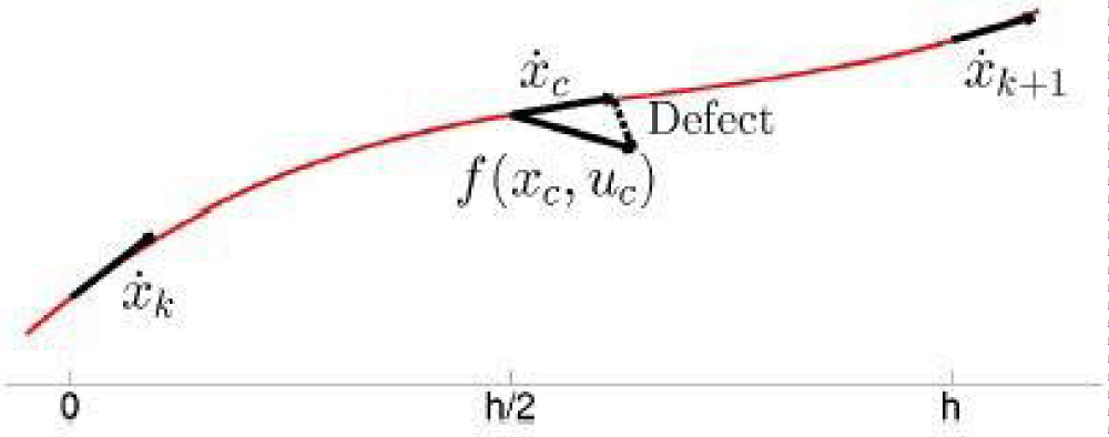
Defects constraints: The difference between the first derivative of the interpolating polynomial at the midpoint of a segment and the first derivative calculated from the equations of motion at the segment midpoint is used as the defect. To have a good approximation of the actual states the defects must approach zero and thus interpolating polynomial is a good approximation, the defect is written in the following form:

ζ j = X ˙ ( τ j )f(x( τ j ), τ j ),      (3.6) MathType@MTEF@5@5@+=feaaguart1ev2aaatCvAUfeBSjuyZL2yd9gzLbvyNv2CaerbuLwBLnhiov2DGi1BTfMBaeXatLxBI9gBaerbd9wDYLwzYbItLDharqqtubsr4rNCHbGeaGqiVu0Je9sqqrpepC0xbbL8F4rqqrFfpeea0xe9Lq=Jc9vqaqpepm0xbba9pwe9Q8fs0=yqaqpepae9pg0FirpepeKkFr0xfr=xfr=xb9adbaqaaeGaciGaaiaabeqaamaabaabaaGcbaaeaaaaaaaaa8qacqaH2oGEpaWaaSbaaSqaa8qacaWGQbaapaqabaGcpeGaeyypa0JabmiwayaacaGaaiikaiabes8a09aadaWgaaWcbaWdbiaadQgaa8aabeaak8qacaGGPaGaeyOeI0IaamOzaiaacIcacaWG4bGaaiikaiabes8a09aadaWgaaWcbaWdbiaadQgaa8aabeaak8qacaGGPaGaaiilaiabes8a09aadaWgaaWcbaWdbiaadQgaa8aabeaak8qacaGGPaGaaiilaiaabccacaqGGaGaaeiiaiaabccacaqGGaGaaeiiaiaabIcacaqGZaGaaeOlaiaabAdacaqGPaaaaa@541F@

the defect constraint for the trapezoidal method (by setting P( x )=x( τ j ) h j 2 ( f j + f j+1 ) MathType@MTEF@5@5@+=feaaguart1ev2aaatCvAUfeBSjuyZL2yd9gzLbvyNv2CaerbuLwBLnhiov2DGi1BTfMBaeXatLxBI9gBaerbd9wDYLwzYbItLDharqqtubsr4rNCHbGeaGqiVu0Je9sqqrpepC0xbbL8F4rqqrFfpeea0xe9Lq=Jc9vqaqpepm0xbba9pwe9Q8fs0=yqaqpepae9pg0FirpepeKkFr0xfr=xfr=xb9adbaqaaeGaciGaaiaabeqaamaabaabaaGcbaqcaaeeaaaaaaaaa8qacaWGqbGcdaqadaqcaa0daeaapeGaamiEaaGaayjkaiaawMcaaiabg2da9iaadIhakmaabmaajaaqpaqaa8qacqaHepaDk8aadaWgaaqcbauaa8qacaWGQbaapaqabaaajaaqpeGaayjkaiaawMcaaiabgkHiTOWaaSaaaKaaa9aabaWdbiaadIgak8aadaWgaaqcbauaa8qacaWGQbaapaqabaaajaaqbaWdbiaaikdaaaGcdaqadaqcaa0daeaapeGaamOzaOWdamaaBaaajeaqbaWdbiaadQgaa8aabeaajaaqpeGaey4kaSIaamOzaOWdamaaBaaajeaqbaWdbiaadQgacqGHRaWkcaaIXaaapaqabaaajaaqpeGaayjkaiaawMcaaaaa@50FF@ and x i+1 =x( τ j+1 ) MathType@MTEF@5@5@+=feaaguart1ev2aaatCvAUfeBSjuyZL2yd9gzLbvyNv2CaerbuLwBLnhiov2DGi1BTfMBaeXatLxBI9gBaerbd9wDYLwzYbItLDharqqtubsr4rNCHbGeaGqiVu0Je9sqqrpepC0xbbL8F4rqqrFfpeea0xe9Lq=Jc9vqaqpepm0xbba9pwe9Q8fs0=yqaqpepae9pg0FirpepeKkFr0xfr=xfr=xb9adbaqaaeGaciGaaiaabeqaamaabaabaaGcbaaeaaaaaaaaa8qacaWG4bWdamaaBaaaleaapeGaamyAaiabgUcaRiaaigdaa8aabeaak8qacqGH9aqpcaWG4bWaaeWaa8aabaWdbiabes8a09aadaWgaaWcbaWdbiaadQgacqGHRaWkcaaIXaaapaqabaaak8qacaGLOaGaayzkaaaaaa@427E@ at Eq.(3.10))

is defined as:

ζ j ( τ j )=x( τ j+1 )x( τ j ) h j 2 ( f j + f j+1 )=0, MathType@MTEF@5@5@+=feaaguart1ev2aaatCvAUfeBSjuyZL2yd9gzLbvyNv2CaerbuLwBLnhiov2DGi1BTfMBaeXatLxBI9gBaerbd9wDYLwzYbItLDharqqtubsr4rNCHbGeaGqiVu0Je9sqqrpepC0xbbL8F4rqqrFfpeea0xe9Lq=Jc9vqaqpepm0xbba9pwe9Q8fs0=yqaqpepae9pg0FirpepeKkFr0xfr=xfr=xb9adbaqaaeGaciGaaiaabeqaamaabaabaaGcbaaeaaaaaaaaa8qacqaH2oGEpaWaaSbaaSqaa8qacaWGQbaapaqabaGcpeWaaeWaa8aabaWdbiabes8a09aadaWgaaWcbaWdbiaadQgaa8aabeaaaOWdbiaawIcacaGLPaaacqGH9aqpcaWG4bWaaeWaa8aabaWdbiabes8a09aadaWgaaWcbaWdbiaadQgacqGHRaWkcaaIXaaapaqabaaak8qacaGLOaGaayzkaaGaeyOeI0IaamiEamaabmaapaqaa8qacqaHepaDpaWaaSbaaSqaa8qacaWGQbaapaqabaaak8qacaGLOaGaayzkaaGaeyOeI0YaaSaaa8aabaWdbiaadIgapaWaaSbaaSqaa8qacaWGQbaapaqabaaakeaapeGaaGOmaaaadaqadaWdaeaapeGaamOza8aadaWgaaWcbaWdbiaadQgaa8aabeaak8qacqGHRaWkcaWGMbWdamaaBaaaleaapeGaamOAaiabgUcaRiaaigdaa8aabeaaaOWdbiaawIcacaGLPaaacqGH9aqpcaaIWaGaaiilaaaa@5C87@

the defect constraint for the Hermite–Simpson’s method (by setting P(x)=x( τ j ) h k 6 ( f j +4 f ¯ j + f j+1 ) MathType@MTEF@5@5@+=feaaguart1ev2aqatCvAUfeBSjuyZL2yd9gzLbvyNv2CaerbuLwBLnhiov2DGi1BTfMBaeXatLxBI9gBaerbd9wDYLwzYbItLDharqqtubsr4rNCHbGeaGqiVu0Je9sqqrpepC0xbbL8F4rqqrFfpeea0xe9Lq=Jc9vqaqpepm0xbba9pwe9Q8fs0=yqaqpepae9pg0FirpepeKkFr0xfr=xfr=xb9adbaqaaeGaciGaaiaabeqaamaabaabaaGcbaaeaaaaaaaaa8qacaWGqbGaaiikaiaadIhacaGGPaGaeyypa0JaamiEaiaacIcacqaHepaDpaWaaSbaaSqaa8qacaWGQbaapaqabaGcpeGaaiykaiabgkHiTmaalaaapaqaa8qacaWGObWdamaaBaaaleaapeGaam4AaaWdaeqaaaGcbaWdbiaaiAdaaaGaaiikaiaadAgapaWaaSbaaSqaa8qacaWGQbaapaqabaGcpeGaey4kaSIaaGinaiqadAgagaqea8aadaWgaaWcbaWdbiaadQgaa8aabeaak8qacqGHRaWkcaWGMbWdamaaBaaaleaapeGaamOAaiabgUcaRiaaigdaa8aabeaak8qacaGGPaaaaa@5069@ and x   i+1  =x(   τ i+1   ) ) MathType@MTEF@5@5@+=feaaguart1ev2aaatCvAUfeBSjuyZL2yd9gzLbvyNv2CaerbuLwBLnhiov2DGi1BTfMBaeXatLxBI9gBaerbd9wDYLwzYbItLDharqqtubsr4rNCHbGeaGqiVu0Je9sqqrpepC0xbbL8F4rqqrFfpeea0xe9Lq=Jc9vqaqpepm0xbba9pwe9Q8fs0=yqaqpepae9pg0FirpepeKkFr0xfr=xfr=xb9adbaqaaeGaciGaaiaabeqaamaabaabaaGcbaaeaaaaaaaaa8qacaWG4bGaaeiiamaaBaaaleaacaWGPbGaey4kaSIaaGymaaqabaGccaqGGaGaeyypa0JaamiEa8aadaqadaqaa8qacaqGGaGaeqiXdq3aaSbaaSqaaiaadMgacqGHRaWkcaaIXaaabeaakiaabccaa8aacaGLOaGaayzkaaWdbiaabccapaGaaiykaaaa@460B@ at Eq.(3.6) is defined as:

let τ ¯ j =( τ j + τ j+1 )/2,and u ¯ ( τ ¯ j )=( u( τ j )+u( τ +1 ) )/2, MathType@MTEF@5@5@+=feaaguart1ev2aaatCvAUfeBSjuyZL2yd9gzLbvyNv2CaerbuLwBLnhiov2DGi1BTfMBaeXatLxBI9gBaerbd9wDYLwzYbItLDharqqtubsr4rNCHbGeaGqiVu0Je9sqqrpepC0xbbL8F4rqqrFfpeea0xe9Lq=Jc9vqaqpepm0xbba9pwe9Q8fs0=yqaqpepae9pg0FirpepeKkFr0xfr=xfr=xb9adbaqaaeGaciGaaiaabeqaamaabaabaaGcbaaeaaaaaaaaa8qacuaHepaDpaGbaebapeWaaSbaaSqaaiaadQgaaeqaaOGaeyypa0ZaaeWaa8aabaWdbiabes8a09aadaWgaaWcbaWdbiaadQgaa8aabeaak8qacqGHRaWkcqaHepaDpaWaaSbaaSqaa8qacaWGQbGaey4kaSIaaGymaaWdaeqaaaGcpeGaayjkaiaawMcaaiaac+cacaaIYaGaaiila8aacaaMe8UaaG5bV=qacaWGHbGaamOBaiaadsgapaWaa0aaaeaacaaMe8UaaG5bV=qacaWG1baaaiaacIcacuaHepaDpaGbaebapeWaaSbaaSqaaiaadQgaaeqaaOGaaiykaiabg2da9maabmaapaqaa8qacaWG1bWaaeWaa8aabaWdbiabes8a09aadaWgaaWcbaWdbiaadQgaa8aabeaaaOWdbiaawIcacaGLPaaacqGHRaWkcaWG1bWaaeWaa8aabaWdbiabes8a09aadaWgaaWcbaWdbiabgUcaRiaaigdaa8aabeaaaOWdbiaawIcacaGLPaaaaiaawIcacaGLPaaacaGGVaGaaGOmaiaacYcaaaa@677F@ x ˜ ( τ j ¯ ) = 1 2 [x( τ j )+x( τ j+1 )] + h k 8 ( f j f j+1 ), f ¯ j = f[ x ˜ ( τ ¯ j ), u ¯ ( τ j ),p, τ ¯ j ] , ζ( t j ) = x( τ j+1 )x( τ j ) + h k 6 ( f j +4 f ¯ j + f j+1 )=0. MathType@MTEF@5@5@+=feaaguart1ev2aaatCvAUfeBSjuyZL2yd9gzLbvyNv2CaerbuLwBLnhiov2DGi1BTfMBaeXatLxBI9gBaerbd9wDYLwzYbItLDharqqtubsr4rNCHbGeaGqiVu0Je9sqqrpepC0xbbL8F4rqqrFfpeea0xe9Lq=Jc9vqaqpepm0xbba9pwe9Q8fs0=yqaqpepae9pg0FirpepeKkFr0xfr=xfr=xb9adbaqaaeGaciGaaiaabeqaamaabaabaaGcbaqcaawbaeaaboabaaaabaaeaaaaaaaaa8qaceqG4bGbaGaacaGGOaGcdaqdaaqcaa2daeaapeGaeqiXdqNcpaWaaSbaaKqaGfaapeGaaeOAaaWdaeqaaaaajaaypeGaaiykaaWdaeaacqGH9aqpaeaak8qadaWcaaqcaa2daeaapeGaaGymaaWdaeaapeGaaGOmaaaacaGGBbGaamiEaiaacIcacqaHepaDk8aadaWgaaqcbawaa8qacaWGQbaapaqabaqcaa2dbiaacMcacqGHRaWkcaWG4bGaaiikaiabes8a0PWdamaaBaaajeaybaWdbiaadQgacqGHRaWkcaaIXaaapaqabaqcaa2dbiaacMcacaGGDbaapaqaaiabgUcaROWdbmaalaaajaaypaqaa8qacaWGObGcpaWaaSbaaKqaGfaapeGaam4AaaWdaeqaaaqcaawaa8qacaaI4aaaaiaacIcacaWGMbGcpaWaaSbaaKqaGfaapeGaamOAaaWdaeqaaKaaG9qacqGHsislcaWGMbGcpaWaaSbaaKqaGfaapeGaamOAaiabgUcaRiaaigdaa8aabeaajaaypeGaaiykaiaacYcaa8aabaWdbiqadAgagaqeaOWdamaaBaaajeaybaWdbiaadQgaa8aabeaaaKaaGfaacqGH9aqpaeaapeGaamOzaiaacUfaceqG4bGbaGaacaGGOaGafqiXdqNbaebak8aadaWgaaqcbawaa8qacaqGQbaapaqabaqcaa2dbiaacMcacaGGSaGabeyDayaaraGaaeikaiabes8a0PWdamaaBaaajeaybaWdbiaabQgaa8aabeaajaaypeGaaiykaiaacYcacaqGWbGaaiilaiqbes8a0zaaraGcpaWaaSbaaKqaGfaapeGaaeOAaaWdaeqaaKaaG9qacaGGDbaapaqaaiaacYcaaeaapeGaeqOTdONaaiikaiaadshak8aadaWgaaqcbawaa8qacaWGQbaapaqabaqcaa2dbiaacMcaa8aabaGaeyypa0dabaWdbiaadIhacaGGOaGaeqiXdqNcpaWaaSbaaKqaGfaapeGaamOAaiabgUcaRiaaigdaa8aabeaajaaypeGaaiykaiabgkHiTiaadIhacaGGOaGaeqiXdqNcpaWaaSbaaKqaGfaapeGaamOAaaWdaeqaaKaaG9qacaGGPaaapaqaaiabgUcaROWdbmaalaaajaaypaqaa8qacaWGObGcpaWaaSbaaKqaGfaapeGaam4AaaWdaeqaaaqcaawaa8qacaaI2aaaaiaacIcacaWGMbGcpaWaaSbaaKqaGfaapeGaamOAaaWdaeqaaKaaG9qacqGHRaWkcaaI0aGabmOzayaaraGcpaWaaSbaaKqaGfaapeGaamOAaaWdaeqaaKaaG9qacqGHRaWkcaWGMbGcpaWaaSbaaKqaGfaapeGaamOAaiabgUcaRiaaigdaa8aabeaajaaypeGaaiykaiabg2da9iaaicdacaGGUaaaaaaa@AB38@

• The quadrature rule used for integration is consistent with the numerical method used for solving the differential equa- tion. If one is using a Runge-Kutta method for solving the differential equation, the cost would also be approximated using Runge-Kutta integration. In the case of an Hermite–Simpson’s collocation method, the integration rule is Her- mite–Simpson collocated quadrature rule [33].

• Thus the optimal control problem Eq.(3.1) is rewritten as: let si be values of state vector at at grid point, i which represent the states at the collocation points in each subinterval.

min J=φ(x( t 0 ), q 0 , s 0 , t 0 ,x( t f ),q, t f ) + i=0 N1 g (x(t, q i , s i , s ^ i ),u(t, q i , s i , s ^ i )), subject to s 0 x 0 =0, (initial value), s i+1 x i ( t i+1 ; s i , s ^ i , q i ) =0, (continuity), C(x( t i , q i , s i , s ^ i ,),u( t i , q i , s i , s ^ i )) 0, (discretized path constraints), E(x( t 0 ), q 0 , s 0 , t 0 ,x( t f ), q N , s N , t f ) =0. (terminal constraints). MathType@MTEF@5@5@+=feaaguart1ev2aaatCvAUfeBSjuyZL2yd9gzLbvyNv2CaerbuLwBLnhiov2DGi1BTfMBaeXatLxBI9gBaerbd9wDYLwzYbItLDharqqtubsr4rNCHbGeaGqiVu0Je9sqqrpepC0xbbL8F4rqqrFfpeea0xe9Lq=Jc9vqaqpepm0xbba9pwe9Q8fs0=yqaqpepae9pg0FirpepeKkFr0xfr=xfr=xb9adbaqaaeGaciGaaiaabeqaamaabaabaaGcbaaeaaaaaaaaa8qafaqaaeObeaaaaaqaaiGac2gacaGGPbGaaiOBaaqaaiaadQeacqGH9aqpcqaHgpGAcaGGOaGaamiEaiaacIcacaWG0bWdamaaBaaaleaapeGaaGimaaWdaeqaaOWdbiaacMcacaGGSaGaaCyCa8aadaWgaaWcbaWdbiaahcdaa8aabeaak8qacaGGSaGaaC4Ca8aadaWgaaWcbaWdbiaahcdaa8aabeaak8qacaGGSaGaamiDa8aadaWgaaWcbaWdbiaaicdaa8aabeaak8qacaGGSaGaamiEaiaacIcacaWG0bWdamaaBaaaleaapeGaamOzaaWdaeqaaOWdbiaacMcacaGGSaGaaCyCaiaacYcacaWG0bWdamaaBaaaleaapeGaamOzaaWdaeqaaOWdbiaacMcaaeaacqGHRaWkaeaadaaeWbWdaeaacaWGNbaaleaapeGaamyAaiabg2da9iaaicdaa8aabaWdbiaad6eacqGHsislcaaIXaaaniabggHiLdGccaGGOaGaamiEaiaacIcacaWG0bGaaiilaiaahghapaWaaSbaaSqaa8qacaWHPbaapaqabaGcpeGaaiilaiaahohapaWaaSbaaSqaa8qacaWHPbaapaqabaGcpeGaaiilaiqahohagaqca8aadaWgaaWcbaWdbiaahMgaa8aabeaak8qacaGGPaGaaiilaiaadwhacaGGOaGaamiDaiaacYcacaWHXbWdamaaBaaaleaapeGaaCyAaaWdaeqaaOWdbiaacYcacaWHZbWdamaaBaaaleaapeGaaCyAaaWdaeqaaOWdbiaacYcaceWHZbGbaKaapaWaaSbaaSqaa8qacaWHPbaapaqabaGcpeGaaiykaiaacMcacaGGSaaabaaabaGaae4CaiaabwhacaqGIbGaaeOAaiaabwgacaqGJbGaaeiDaiaabccacaqG0bGaae4BaaqaaaqaaaqaaaqaaiaadohadaWgaaWcbaGaaGimaaqabaGccqGHsislcaWG4bWaaSbaaSqaaiaaicdaaeqaaaGcbaGaeyypa0JaaGimaiaacYcaaeaacaGGOaGaaeyAaiaab6gacaqGPbGaaeiDaiaabMgacaqGHbGaaeiBaiaabccacaqG2bGaaeyyaiaabYgacaqG1bGaaeyzaiaabMcacaqGSaaabaaabaGaaC4Ca8aadaWgaaWcbaWdbiaahMgacqGHRaWkcaWHXaaapaqabaGcpeGaeyOeI0IaaCiEa8aadaWgaaWcbaWdbiaahMgaa8aabeaak8qacaGGOaGaaCiDa8aadaWgaaWcbaWdbiaahMgacqGHRaWkcaWHXaaapaqabaGcpeGaai4oaiaahohapaWaaSbaaSqaa8qacaWHPbaapaqabaGcpeGaaiilaiqahohagaqca8aadaWgaaWcbaWdbiaahMgaa8aabeaak8qacaGGSaGaaCyCa8aadaWgaaWcbaWdbiaahMgaa8aabeaak8qacaGGPaaabaGaeyypa0JaaGimaiaacYcaaeaacaGGOaGaae4yaiaab+gacaqGUbGaaeiDaiaabMgacaqGUbGaaeyDaiaabMgacaqG0bGaaeyEaiaacMcacaGGSaaabaaabaGaam4qaiaacIcacaWG4bGaaiikaiaadshapaWaaSbaaSqaa8qacaWGPbaapaqabaGcpeGaaiilaiaahghapaWaaSbaaSqaa8qacaWHPbaapaqabaGcpeGaaiilaiaahohapaWaaSbaaSqaa8qacaWHPbaapaqabaGcpeGaaiilaiqahohagaqca8aadaWgaaWcbaWdbiaahMgaa8aabeaak8qacaGGSaGaaiykaiaacYcacaWG1bGaaiikaiaadshapaWaaSbaaSqaa8qacaWGPbaapaqabaGcpeGaaiilaiaahghapaWaaSbaaSqaa8qacaWHPbaapaqabaGcpeGaaiilaiaahohapaWaaSbaaSqaa8qacaWHPbaapaqabaGcpeGaaiilaiqahohagaqca8aadaWgaaWcbaWdbiaahMgaa8aabeaak8qacaGGPaGaaiykaaqaaiabgsMiJkaaicdacaGGSaaabaGaaiikaiaabsgacaqGPbGaae4CaiaabogacaqGYbGaaeyzaiaabshacaqGPbGaaeOEaiaabwgacaqGKbGaaeiiaiaabchacaqGHbGaaeiDaiaabIgapaGaaG5bVlaabccapeGaae4yaiaab+gacaqGUbGaae4CaiaabshacaqGYbGaaeyyaiaabMgacaqGUbGaaeiDaiaabohacaqGPaGaaiilaaqaaaqaaiaadweacaGGOaGaamiEaiaacIcacaWG0bWdamaaBaaaleaapeGaaGimaaWdaeqaaOWdbiaacMcacaGGSaGaaCyCa8aadaWgaaWcbaWdbiaahcdaa8aabeaak8qacaGGSaGaaC4Ca8aadaWgaaWcbaWdbiaahcdaa8aabeaak8qacaGGSaGaamiDa8aadaWgaaWcbaWdbiaaicdaa8aabeaak8qacaGGSaGaamiEaiaacIcacaWG0bWdamaaBaaaleaapeGaamOzaaWdaeqaaOWdbiaacMcacaGGSaGaaCyCa8aadaWgaaWcbaWdbiaah6eaa8aabeaak8qacaGGSaGaaC4Ca8aadaWgaaWcbaWdbiaah6eaa8aabeaak8qacaGGSaGaamiDa8aadaWgaaWcbaWdbiaadAgaa8aabeaak8qacaGGPaaabaGaeyypa0JaaGimaiaac6caaeaacaqGOaGaaeiDaiaabwgacaqGYbGaaeyBaiaabMgacaqGUbGaaeyyaiaabYgapaGaaG5bVlaabccapeGaae4yaiaab+gacaqGUbGaae4CaiaabshacaqGYbGaaeyyaiaabMgacaqGUbGaaeiDaiaabohacaqGPaGaaiOlaaaaaaa@32CF@

Solution of the NLP problem

Numerical methods for solving NLPs fall into categories: gradient based (local) methods and heuristic (global) methods, gradient based (local) approach is now described in the following algorithm (the heuristic method is out of the interest of this article, for more details see [40]).

The convergence may depend on a given tolerance or depends on no further change in the objective function after several iterations. There are many ways to modify direction selection and step size, and this leads to many different algorithms. Some of common ones included Steepest Descent Methods, Conjugate Direction Method, Simplex Method, Interior Point Method (IP) and Sequential Quadratic Programming, more details on the IP methods will be given here.

Algorithm 2: Gradient Based Algorithm. Notations: Let z is the unknown decision vector, k is the iteration counter, p is the search direction along which to change the current value zk, αk is the magnitude of the change in zk. 1: while not converged do. 2: Steps are taken in a certain direction i.e., the kth iteration, a search direction is pk and a step length, αk are determined.
The update from zk, to zk+1 has the form: zk+1 = zk + αpk, 3: The objective function is evaluated, in case of minimization, the search direction is chosen to sufficiently decrease the objective function in the form. 4: If the objective function improves take another step at the same direction else change the direction, step size or both. 5: end while.

IP Method: it is typically eliminate constraints of the form h ¯ h(x) h ¯ MathType@MTEF@5@5@+=feaaguart1ev2aaatCvAUfeBSjuyZL2yd9gzLbvyNv2CaerbuLwBLnhiov2DGi1BTfMBaeXatLxBI9gBaerbd9wDYLwzYbItLDharqqtubsr4rNCHbGeaGqiVu0Je9sqqrpepC0xbbL8F4rqqrFfpeea0xe9Lq=Jc9vqaqpepm0xbba9pwe9Q8fs0=yqaqpepae9pg0FirpepeKkFr0xfr=xfr=xb9adbaqaaeGaciGaaiaabeqaamaabaabaaGcbaWaaWaaaeaacaWGObaaaiabgsMiJkaadIgacaGGOaGaamiEaiaacMcacqGHKjYOdaqdaaqaaiaadIgaaaaaaa@3E9A@ by introducing slack variables additional equality constraints. After locating an interior point, i.e., a point where x ¯ <x< x ¯ MathType@MTEF@5@5@+=feaaguart1ev2aaatCvAUfeBSjuyZL2yd9gzLbvyNv2CaerbuLwBLnhiov2DGi1BTfMBaeXatLxBI9gBaerbd9wDYLwzYbItLDharqqtubsr4rNCHbGeaGqiVu0Je9sqqrpepC0xbbL8F4rqqrFfpeea0xe9Lq=Jc9vqaqpepm0xbba9pwe9Q8fs0=yqaqpepae9pg0FirpepeKkFr0xfr=xfr=xb9adbaqaaeGaciGaaiaabeqaamaabaabaaGcbaWaaWaaaeaacaWG4baaaiabgYda8iaadIhacqGH8aapdaqdaaqaaiaadIhaaaaaaa@3B12@ holds with strict inequality, which may require reformulating some decision variables as parameters, they formulate a barrier problem of the form:

min f( x ) μ i=1 n x l og( x ¯ i x i ) + log( x i x ¯ i )), subject to g( x )=0. MathType@MTEF@5@5@+=feaaguart1ev2aaatCvAUfeBSjuyZL2yd9gzLbvyNv2CaerbuLwBLnhiov2DGi1BTfMBaeXatLxBI9gBaerbd9wDYLwzYbItLDharqqtubsr4rNCHbGeaGqiVu0Je9sqqrpepC0xbbL8F4rqqrFfpeea0xe9Lq=Jc9vqaqpepm0xbba9pwe9Q8fs0=yqaqpepae9pg0FirpepeKkFr0xfr=xfr=xb9adbaqaaeGaciGaaiaabeqaamaabaabaaGcbaqbaeaaboGbaaaabaGaciyBaiaacMgacaGGUbaabaaeaaaaaaaaa8qacaWGMbWdamaabmaabaWdbiaadIhaa8aacaGLOaGaayzkaaaabaGaeyOeI0cabaWdbiabeY7aTnaaqahapaqaa8qacaWGSbaal8aabaWdbiaadMgacqGH9aqpcaaIXaaapaqaa8qacaWGUbWdamaaBaaameaapeGaamiEaaWdaeqaaaqdpeGaeyyeIuoakiaad+gacaWGNbGaaiikaiqadIhagaqea8aadaWgaaWcbaWdbiaadMgaa8aabeaak8qacqGHsislcaWG4bWdamaaBaaaleaapeGaamyAaaWdaeqaaOWdbiaacMcaa8aabaGaey4kaScabaWdbiaadYgacaWGVbGaam4zaiaacIcacaWG4bWdamaaBaaaleaapeGaamyAaaWdaeqaaOWdbiabgkHiTiqadIhagaqha8aadaWgaaWcbaWdbiaadMgaa8aabeaak8qacaGGPaGaaiykaiaacYcaa8aabaaabaGaae4CaiaabwhacaqGIbGaaeOAaiaabwgacaqGJbGaaeiDaiaabccacaqG0bGaae4Baaqaaaqaaaqaaaqaaaqaaaqaaaqaaaqaa8qacaWGNbWdamaabmaabaWdbiaadIhaa8aacaGLOaGaayzkaaGaeyypa0JaaGimaiaac6caaeaaaeaaaaaaaa@6D11@

Sequences of barrier problems for increasing values of the barrier parameter µ are then solved with Newton-type methods, for more details see [7,40].

Accuracy

Since the solution obtained from the NLP problem is a discrete set of numbers we don’t know what happen between the discrete points, a continuous approximation to the discrete solution resulted from the NLP is needed, i.e., representing the solution (interpolation) [6].

Spline representation: To get the solution as continuous approximation [ y ˜ (t), u ˜ (t) ] MathType@MTEF@5@5@+=feaaguart1ev2aaatCvAUfeBSjuyZL2yd9gzLbvyNv2CaerbuLwBLnhiov2DGi1BTfMBaeXatLxBI9gBaerbd9wDYLwzYbItLDharqqtubsr4rNCHbGeaGqk0Jf9crFfpeea0xh9v8qiW7rqqrFfpeea0xe9Lq=Jc9vqaqpepm0xbba9pwe9Q8fs0=yqaqpepae9pg0FirpepeKkFr0xfr=xfr=xb9adbaqaaeGaciGaaiaabeqaamaabaabaaGcbaWaamWaaeaadaaiaaqaaiaabMhaaiaawoWaaiaacIcacaWG0bGaaiykaiaacYcadaaiaaqaaiaabwhaaiaawoWaaiaacIcacaWG0bGaaiykaaGaay5waiaaw2faaaaa@42C3@ from the NLP solution we use spline representation (where spline is a sequence i.e., whole collection of polynomial) defined as follows:

[ y(t) u(t) ]=[ y ˜ (t) u ˜ (t) ]= i=1 n 1 α i β i (t),     (3.7) MathType@MTEF@5@5@+=feaaguart1ev2aaatCvAUfeBSjuyZL2yd9gzLbvyNv2CaerbuLwBLnhiov2DGi1BTfMBaeXatLxBI9gBaerbd9wDYLwzYbItLDharqqtubsr4rNCHbGeaGqiVu0Je9sqqrpepC0xbbL8F4rqqrFfpeea0xe9Lq=Jc9vqaqpepm0xbba9pwe9Q8fs0=yqaqpepae9pg0FirpepeKkFr0xfr=xfr=xb9adbaqaaeGaciGaaiaabeqaamaabaabaaGcbaaeaaaaaaaaa8qadaWadaabaeqabaGaamyEaiaacIcacaWG0bGaaiykaaqaaiaadwhacaGGOaGaamiDaiaacMcaaaGaay5waiaaw2faaiabg2da9maadmaaeaqabeaaceWG5bGbaGaacaGGOaGaamiDaiaacMcaaeaaceWG1bGbaGaacaGGOaGaamiDaiaacMcaaaGaay5waiaaw2faaiabg2da9maaqahapaqaa8qacqaHXoqypaWaaSbaaSqaa8qacaWGPbaapaqabaaabaWdbiaadMgacqGH9aqpcaaIXaaapaqaa8qacaWGUbWdamaaBaaameaapeGaaGymaaWdaeqaaaqdpeGaeyyeIuoakiabek7aI9aadaWgaaWcbaWdbiaadMgaa8aabeaak8qacaGGOaGaamiDaiaacMcacaGGSaGaaeiiaiaabccacaqGGaGaaeiiaiaabccacaqGOaGaae4maiaab6cacaqG3aGaaeykaaaa@6050@

where n1 = 2M, M is the number of mesh points, y(t), u(t) are the true state and control respectively, [ y ˜ (t), u ˜ (t) ] MathType@MTEF@5@5@+=feaaguart1ev2aaatCvAUfeBSjuyZL2yd9gzLbvyNv2CaerbuLwBLnhiov2DGi1BTfMBaeXatLxBI9gBaerbd9wDYLwzYbItLDharqqtubsr4rNCHbGeaGqk0Jf9crFfpeea0xh9v8qiW7rqqrFfpeea0xe9Lq=Jc9vqaqpepm0xbba9pwe9Q8fs0=yqaqpepae9pg0FirpepeKkFr0xfr=xfr=xb9adbaqaaeGaciGaaiaabeqaamaabaabaaGcbaWaamWaaeaadaaiaaqaaiaabMhaaiaawoWaaiaacIcacaWG0bGaaiykaiaacYcadaaiaaqaaiaabwhaaiaawoWaaiaacIcacaWG0bGaaiykaaGaay5waiaaw2faaaaa@42C3@ are the approximate state and control respectively, the functions βi(t) form a basis for C0 or C1 cubic B-splines with n1 = 2M, where M is the number of mesh points. The coefficients αi in the state or control variable representation which is defined by different Interpolation of discrete solution depending on the discritization method, the spline approximation Eq. (3.7) must match the state at the grid points i.e.,

y ˜ ( t )= y k ,  for k=1,...,M, MathType@MTEF@5@5@+=feaaguart1ev2aaatCvAUfeBSjuyZL2yd9gzLbvyNv2CaerbuLwBLnhiov2DGi1BTfMBaeXatLxBI9gBaerbd9wDYLwzYbItLDharqqtubsr4rNCHbGeaGqiVu0Je9sqqrpepC0xbbL8F4rqqrFfpeea0xe9Lq=Jc9vqaqpepm0xbba9pwe9Q8fs0=yqaqpepae9pg0FirpepeKkFr0xfr=xfr=xb9adbaqaaeGaciGaaiaabeqaamaabaabaaGcbaaeaaaaaaaaa8qadaaiaaqaaiaadMhaaiaawoWaamaabmaapaqaa8qacaWG0baacaGLOaGaayzkaaGaeyypa0JaamyEa8aadaWgaaWcbaWdbiaadUgaa8aabeaak8qacaGGSaWdaiaayAW7caaMe8UaaG5aV=qacaWGMbGaam4BaiaadkhacaqGGaWdaiaaygW7peGaam4Aaiabg2da9iaaigdacaGGSaGaaiOlaiaac6cacaGGUaGaaiilaiaad2eacaGGSaaaaa@501D@

the derivative of the spline approximation must match the right-hand side of the differential equations,

d dt y ˜ ( t )= f k ,  fork=1,...,M, MathType@MTEF@5@5@+=feaaguart1ev2aaatCvAUfeBSjuyZL2yd9gzLbvyNv2CaerbuLwBLnhiov2DGi1BTfMBaeXatLxBI9gBaerbd9wDYLwzYbItLDharqqtubsr4rNCHbGeaGqiVu0Je9sqqrpepC0xbbL8F4rqqrFfpeea0xe9Lq=Jc9vqaqpepm0xbba9pwe9Q8fs0=yqaqpepae9pg0FirpepeKkFr0xfr=xfr=xb9adbaqaaeGaciGaaiaabeqaamaabaabaaGcbaaeaaaaaaaaa8qadaWcaaWdaeaapeGaamizaaWdaeaapeGaamizaiaadshaaaWaaacaaeaacaWG5baacaGLdmaadaqadaWdaeaapeGaamiDaaGaayjkaiaawMcaaiabg2da9iaadAgapaWaaSbaaSqaa8qacaWGRbaapaqabaGcpeGaaiila8aacaaMg8UaaGjbVlaayoW7peGaamOzaiaad+gacaWGYbWdaiaaysW7caaMh8+dbiaadUgacqGH9aqpcaaIXaGaaiilaiaac6cacaGGUaGaaiOlaiaacYcacaWGnbGaaiilaaaa@5413@

we require the spline approximation in Eq.(3.7) to match the control at the grid points, i.e.,

u ˜ ( t k )= u k ,,  for k=1,...,M, MathType@MTEF@5@5@+=feaaguart1ev2aaatCvAUfeBSjuyZL2yd9gzLbvyNv2CaerbuLwBLnhiov2DGi1BTfMBaeXatLxBI9gBaerbd9wDYLwzYbItLDharqqtubsr4rNCHbGeaGqiVu0Je9sqqrpepC0xbbL8F4rqqrFfpeea0xe9Lq=Jc9vqaqpepm0xbba9pwe9Q8fs0=yqaqpepae9pg0FirpepeKkFr0xfr=xfr=xb9adbaqaaeGaciGaaiaabeqaamaabaabaaGcbaaeaaaaaaaaa8qadaaiaaqaaiaadwhaaiaawoWaamaabmaapaqaa8qacaWG0bWdamaaBaaaleaapeGaam4AaaWdaeqaaaGcpeGaayjkaiaawMcaaiabg2da9iaadwhapaWaaSbaaSqaa8qacaWGRbaapaqabaGcpeGaaiilaiaacYcapaGaaGPbVlaaysW7caaMd8+dbiaadAgacaWGVbGaamOCa8aacaaMb8Uaaeiia8qacaWGRbGaeyypa0JaaGymaiaacYcacaGGUaGaaiOlaiaac6cacaGGSaGaamytaiaacYcaaaa@5229@

the state variable is C1 cubic function whereas the control variable is C0 linear or quadratic functions depending on the discritization method. Since both y ˜ ( t ), u ˜ ( t ) MathType@MTEF@5@5@+=feaaguart1ev2aaatCvAUfeBSjuyZL2yd9gzLbvyNv2CaerbuLwBLnhiov2DGi1BTfMBaeXatLxBI9gBaerbd9wDYLwzYbItLDharqqtubsr4rNCHbGeaGqiVu0Je9sqqrpepC0xbbL8F4rqqrFfpeea0xe9Lq=Jc9vqaqpepm0xbba9pwe9Q8fs0=yqaqpepae9pg0FirpepeKkFr0xfr=xfr=xb9adbaqaaeGaciGaaiaabeqaamaabaabaaGcbaaeaaaaaaaaa8qadaaiaaqaaiaadMhaaiaawoWaamaabmaapaqaa8qacaWG0baacaGLOaGaayzkaaGaaiilamaaGaaabaGaamyDaaGaay5adaWaaeWaa8aabaWdbiaadshaaiaawIcacaGLPaaaaaa@3F80@ are approximate to the true solution the degree to which this approximation approximate the true solution need to be determined which is known as discretization error and relative local error.

Discretization error: by assuming that the computed control is correct and assume the spline solutions y ˜ ( t ), u ˜ ( t ) MathType@MTEF@5@5@+=feaaguart1ev2aaatCvAUfeBSjuyZL2yd9gzLbvyNv2CaerbuLwBLnhiov2DGi1BTfMBaeXatLxBI9gBaerbd9wDYLwzYbItLDharqqtubsr4rNCHbGeaGqiVu0Je9sqqrpepC0xbbL8F4rqqrFfpeea0xe9Lq=Jc9vqaqpepm0xbba9pwe9Q8fs0=yqaqpepae9pg0FirpepeKkFr0xfr=xfr=xb9adbaqaaeGaciGaaiaabeqaamaabaabaaGcbaaeaaaaaaaaa8qadaaiaaqaaiaadMhaaiaawoWaamaabmaapaqaa8qacaWG0baacaGLOaGaayzkaaGaaiilamaaGaaabaGaamyDaaGaay5adaWaaeWaa8aabaWdbiaadshaaiaawIcacaGLPaaaaaa@3F80@ produced from the NLP, and the single interval t k t t k + h k , MathType@MTEF@5@5@+=feaaguart1ev2aaatCvAUfeBSjuyZL2yd9gzLbvyNv2CaerbuLwBLnhiov2DGi1BTfMBaeXatLxBI9gBaerbd9wDYLwzYbItLDharqqtubsr4rNCHbGeaGqiVu0Je9sqqrpepC0xbbL8F4rqqrFfpeea0xe9Lq=Jc9vqaqpepm0xbba9pwe9Q8fs0=yqaqpepae9pg0FirpepeKkFr0xfr=xfr=xb9adbaqaaeGaciGaaiaabeqaamaabaabaaGcbaaeaaaaaaaaa8qacaWG0bWdamaaBaaaleaapeGaam4AaaWdaeqaaOWdbiabgsMiJkaadshacqGHKjYOcaWG0bWdamaaBaaaleaapeGaam4AaaWdaeqaaOWdbiabgUcaRiaadIgapaWaaSbaaSqaa8qacaWGRbaapaqabaGcpeGaaiilaaaa@4312@ from the state equation we can define

y( t k + h k )=y( t k )+ t k t k + h k y ˙ dt=y( t k )+ t k t k + h k f( y,u,t )dt, MathType@MTEF@5@5@+=feaaguart1ev2aaatCvAUfeBSjuyZL2yd9gzLbvyNv2CaerbuLwBLnhiov2DGi1BTfMBaeXatLxBI9gBaerbd9wDYLwzYbItLDharqqtubsr4rNCHbGeaGqiVu0Je9sqqrpepC0xbbL8F4rqqrFfpeea0xe9Lq=Jc9vqaqpepm0xbba9pwe9Q8fs0=yqaqpepae9pg0FirpepeKkFr0xfr=xfr=xb9adbaqaaeGaciGaaiaabeqaamaabaabaaGcbaaeaaaaaaaaa8qacaWG5bWaaeWaa8aabaWdbiaadshapaWaaSbaaSqaa8qacaWGRbaapaqabaGcpeGaey4kaSIaamiAa8aadaWgaaWcbaWdbiaadUgaa8aabeaaaOWdbiaawIcacaGLPaaacqGH9aqpcaWG5bWaaeWaa8aabaWdbiaadshapaWaaSbaaSqaa8qacaWGRbaapaqabaaak8qacaGLOaGaayzkaaGaey4kaSIaey4kIi=damaaDaaaleaapeGaamiDa8aadaWgaaadbaWdbiaadUgaa8aabeaaaSqaa8qacaWG0bWdamaaBaaameaapeGaam4AaaWdaeqaaSWdbiabgUcaRiaadIgapaWaaSbaaWqaa8qacaWGRbaapaqabaaaaOWdbiqadMhapaGbaiaapeGaaeizaiaadshacqGH9aqpcaWG5bWaaeWaa8aabaWdbiaadshapaWaaSbaaSqaa8qacaWGRbaapaqabaaak8qacaGLOaGaayzkaaGaey4kaSIaey4kIi=damaaDaaaleaapeGaamiDa8aadaWgaaadbaWdbiaadUgaa8aabeaaaSqaa8qacaWG0bWdamaaBaaameaapeGaam4AaaWdaeqaaSWdbiabgUcaRiaadIgapaWaaSbaaWqaa8qacaWGRbaapaqabaaaaOWdbiaadAgadaqadaWdaeaapeGaamyEaiaacYcacaWG1bGaaiilaiaadshaaiaawIcacaGLPaaapaGaaGjbVlaayEW7peGaaeizaiaadshacaGGSaaaaa@6FE6@

where y and u are the true state and control values, we can consider the approximation:

y ^ ( t k + h k )=y( t k )+ t k t k + h k f [ y ˜ (t), u ˜ (t),t]dt,      (3.8) MathType@MTEF@5@5@+=feaaguart1ev2aqatCvAUfeBSjuyZL2yd9gzLbvyNv2CaerbuLwBLnhiov2DGi1BTfMBaeXatLxBI9gBaerbd9wDYLwzYbItLDharqqtubsr4rNCHbGeaGqiVu0Je9sqqrpepC0xbbL8F4rqqrFfpeea0xe9Lq=Jc9vqaqpepm0xbba9pwe9Q8fs0=yqaqpepae9pg0FirpepeKkFr0xfr=xfr=xb9adbaqaaeGaciGaaiaabeqaamaabaabaaGcbaaeaaaaaaaaa8qaceWG5bGbaKaacaGGOaGaamiDa8aadaWgaaWcbaWdbiaadUgaa8aabeaak8qacqGHRaWkcaWGObWdamaaBaaaleaapeGaam4AaaWdaeqaaOWdbiaacMcacqGH9aqpcaWG5bGaaiikaiaadshapaWaaSbaaSqaa8qacaWGRbaapaqabaGcpeGaaiykaiabgUcaRmaapedapaqaa8qacaWGMbaal8aabaWdbiaadshapaWaaSbaaWqaa8qacaWGRbaapaqabaaaleaapeGaamiDa8aadaWgaaadbaWdbiaadUgaa8aabeaal8qacqGHRaWkcaWGObWdamaaBaaameaapeGaam4AaaWdaeqaaaqdpeGaey4kIipakiaacUfaceWG5bGbaGaacaGGOaGaamiDaiaacMcacaGGSaGabmyDayaaiaGaaiikaiaadshacaGGPaGaaiilaiaadshacaGGDbGaamizaiaadshacaGGSaGaaeiiaiaabccacaqGGaGaaeiiaiaabccacaqGGaGaaeikaiaabodacaqGUaGaaeioaiaabMcaaaa@649A@

from Eq.(3.8) we can define the discretization error on the Kth mesh iteration as:

η k = max i { a i | y ˜ i ( t k + h k ) y i ( t k + h k ) |}, MathType@MTEF@5@5@+=feaaguart1ev2aaatCvAUfeBSjuyZL2yd9gzLbvyNv2CaerbuLwBLnhiov2DGi1BTfMBaeXatLxBI9gBaerbd9wDYLwzYbItLDharqqtubsr4rNCHbGeaGqiVu0Je9sqqrpepC0xbbL8F4rqqrFfpeea0xe9Lq=Jc9vqaqpepm0xbba9pwe9Q8fs0=yqaqpepae9pg0FirpepeKkFr0xfr=xfr=xb9adbaqaaeGaciGaaiaabeqaamaabaabaaGcbaaeaaaaaaaaa8qacqaH3oaApaWaaSbaaSqaa8qacaWGRbaapaqabaGcpeGaeyypa0ZdamaaxababaWdbiGac2gacaGGHbGaaiiEaaWcpaqaa8qacaWGPbaapaqabaGccaGG7bWdbiaadggapaWaaSbaaSqaa8qacaWGPbaapaqabaGcpeWaaqWaa8aabaGabmyEayaaiaWaaSbaaSqaa8qacaWGPbaapaqabaGcpeWaaeWaa8aabaWdbiaadshapaWaaSbaaSqaa8qacaWGRbaapaqabaGcpeGaey4kaSIaamiAa8aadaWgaaWcbaWdbiaadUgaa8aabeaaaOWdbiaawIcacaGLPaaacqGHsislceWG5bGbambadaWgaaWcbaGaamyAaaqabaGcdaqadaWdaeaapeGaamiDa8aadaWgaaWcbaWdbiaadUgaa8aabeaak8qacqGHRaWkcaWGObWdamaaBaaaleaapeGaam4AaaWdaeqaaaGcpeGaayjkaiaawMcaaaGaay5bSlaawIa7a8aacaGG9bWdbiaacYcaaaa@5ACB@

For i=1,2,...,n, MathType@MTEF@5@5@+=feaaguart1ev2aaatCvAUfeBSjuyZL2yd9gzLbvyNv2CaerbuLwBLnhiov2DGi1BTfMBaeXatLxBI9gBaerbd9wDYLwzYbItLDharqqtubsr4rNCHbGeaGqiVu0Je9sqqrpepC0xbbL8F4rqqrFfpeea0xe9Lq=Jc9vqaqpepm0xbba9pwe9Q8fs0=yqaqpepae9pg0FirpepeKkFr0xfr=xfr=xb9adbaqaaeGaciGaaiaabeqaamaabaabaaGcbaaeaaaaaaaaa8qacaWGPbGaeyypa0JaaGymaiaacYcacaaIYaGaaiilaiaac6cacaGGUaGaaiOlaiaacYcacaWGUbGaaiilaaaa@3F46@ where the weights ai are chosen to appropriately normalize the error.

Relative local error: is the maximum relative error over all components i in the state equations y˙_ f evaluated in the interval k, and is defined as

ϵ k max i η i,k ( w i +1 ) , MathType@MTEF@5@5@+=feaaguart1ev2aaatCvAUfeBSjuyZL2yd9gzLbvyNv2CaerbuLwBLnhiov2DGi1BTfMBaeXatLxBI9gBaerbd9wDYLwzYbItLDharqqtubsr4rNCHbGeaGqiVu0Je9sqqrpepC0xbbL8F4rqqrFfpeea0xe9Lq=Jc9vqaqpepm0xbba9pwe9Q8fs0=yqaqpepae9pg0FirpepeKkFr0xfr=xfr=xb9adbaqaaeGaciGaaiaabeqaamaabaabaaGcbaWefv3ySLgznfgDOfdaryqr1ngBPrginfgDObYtUvgaiuGaqaaaaaaaaaWdbiab=v=aY=aadaWgaaWcbaWdbiaadUgaa8aabeaak8qacqGHijYUpaWaaCbeaeaapeGaciyBaiaacggacaGG4baal8aabaWdbiaadMgaa8aabeaak8qadaWcaaWdaeaapeGaeq4TdG2damaaBaaaleaapeGaamyAaiaacYcacaWGRbaapaqabaaakeaapeWaaeWaa8aabaWdbiaadEhapaWaaSbaaSqaa8qacaWGPbaapaqabaGcpeGaey4kaSIaaGymaaGaayjkaiaawMcaaaaacaGGSaaaaa@54B4@

where the scale weight w i = max k=1 M [ | y ˜ i,k | , | y ˜ ˙ i,k | ], MathType@MTEF@5@5@+=feaaguart1ev2aaatCvAUfeBSjuyZL2yd9gzLbvyNv2CaerbuLwBLnhiov2DGi1BTfMBaeXatLxBI9gBaerbd9wDYLwzYbItLDharqqtubsr4rNCHbGeaGqiVu0Je9sqqrpepC0xbbL8F4rqqrFfpeea0xe9Lq=Jc9vqaqpepm0xbba9pwe9Q8fs0=yqaqpepae9pg0FirpepeKkFr0xfr=xfr=xb9adbaqaaeGaciGaaiaabeqaamaabaabaaGcbaaeaaaaaaaaa8qacaWG3bWdamaaBaaaleaapeGaamyAaaWdaeqaaOWdbiabg2da98aadaWfWaqaa8qaciGGTbGaaiyyaiaacIhaaSWdaeaapeGaam4Aaiabg2da9iaaigdaa8aabaWdbiaad2eaaaGcdaWadaWdaeaapeWaaqWaa8aabaGabmyEayaaiaWaaSbaaSqaa8qacaWGPbGaaiilaiaadUgaa8aabeaak8qadaabdaWdaeaapeGaaiilaaGaay5bSlaawIa7aiqadMhagaacgaGaa8aadaWgaaWcbaWdbiaadMgacaGGSaGaam4AaaWdaeqaaaGcpeGaay5bSlaawIa7aaGaay5waiaaw2faaiaacYcaaaa@5286@ defines the maximum value for the ith state variable or its derivative over the M grid points in the phase. An equivalent form can be defined as follows the absolute local error on a particular step by

η i,k = t k t k+1 | ε i (s) | ds,      (3.9) MathType@MTEF@5@5@+=feaaguart1ev2aqatCvAUfeBSjuyZL2yd9gzLbvyNv2CaerbuLwBLnhiov2DGi1BTfMBaeXatLxBI9gBaerbd9wDYLwzYbItLDharqqtubsr4rNCHbGeaGqiVu0Je9sqqrpepC0xbbL8F4rqqrFfpeea0xe9Lq=Jc9vqaqpepm0xbba9pwe9Q8fs0=yqaqpepae9pg0FirpepeKkFr0xfr=xfr=xb9adbaqaaeGaciGaaiaabeqaamaabaabaaGcbaaeaaaaaaaaa8qacqaH3oaApaWaaSbaaSqaa8qacaWGPbGaaiilaiaadUgaa8aabeaak8qacqGH9aqpdaWdXaWdaeaapeWaaqWaa8aabaWdbiabew7aL9aadaWgaaWcbaWdbiaadMgaa8aabeaak8qacaGGOaGaam4CaiaacMcaaiaawEa7caGLiWoaaSWdaeaapeGaamiDa8aadaWgaaadbaWdbiaadUgaa8aabeaaaSqaa8qacaWG0bWdamaaBaaameaapeGaam4AaiabgUcaRiaaigdaa8aabeaaa0WdbiabgUIiYdGccaWGKbGaam4CaiaacYcacaqGGaGaaeiiaiaabccacaqGGaGaaeiiaiaabccacaqGOaGaae4maiaab6cacaqG5aGaaeykaaaa@5700@

Where ε( t )= y ˜ ˙ ( t )f[ y ˜ ( t ), u ˜ ( t ),t ] MathType@MTEF@5@5@+=feaaguart1ev2aaatCvAUfeBSjuyZL2yd9gzLbvyNv2CaerbuLwBLnhiov2DGi1BTfMBaeXatLxBI9gBaerbd9wDYLwzYbItLDharqqtubsr4rNCHbGeaGqiVu0Je9sqqrpepC0xbbL8F4rqqrFfpeea0xe9Lq=Jc9vqaqpepm0xbba9pwe9Q8fs0=yqaqpepae9pg0FirpepeKkFr0xfr=xfr=xb9adbaqaaeGaciGaaiaabeqaamaabaabaaGcbaaeaaaaaaaaa8qacqaH1oqzdaqadaWdaeaapeGaamiDaaGaayjkaiaawMcaaiabg2da9iqadMhagaacgaGaamaabmaapaqaa8qacaWG0baacaGLOaGaayzkaaGaeyOeI0IaamOzamaadmaapaqaa8qaceWG5bGbaGaadaqadaWdaeaapeGaamiDaaGaayjkaiaawMcaaiaacYcaceWG1bGbaGaadaqadaWdaeaapeGaamiDaaGaayjkaiaawMcaaiaacYcacaWG0baacaGLBbGaayzxaaaaaa@4CB0@ defines the error in the differential equation as a function of t. An accurate estimate for the integral in Eq.(3.9) is evaluated by using a standard quadrature method, (i.e., Romberg quadrature algorithm).

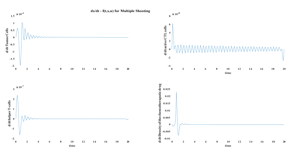
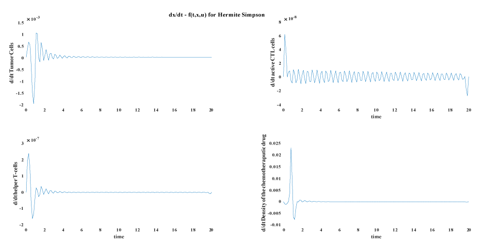
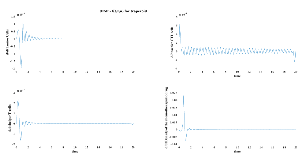
In this part we compare the results from the our base line article [37], with another indirect method solved by sweep method [27] and another three direct method namely direct multiple shooting, trapezoidal direct collocation and Hermite–Simpsons’s direct collocation.
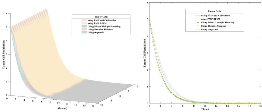

Download Image

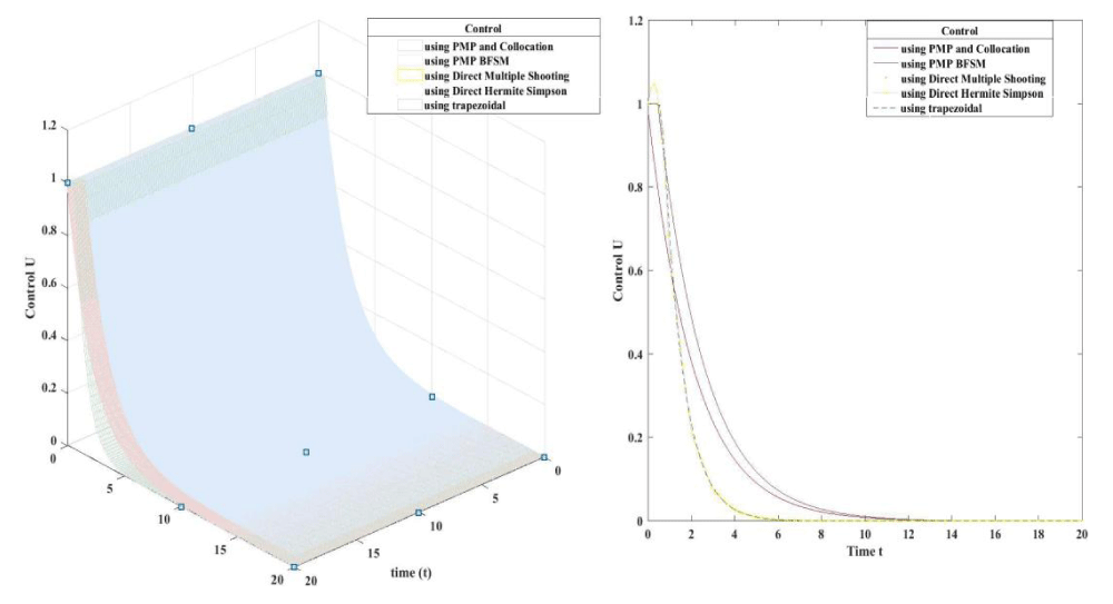
Figure 4.1: Tumor Cell population using 3D plot (left figure) and 2D plot (right figure).


Download Image

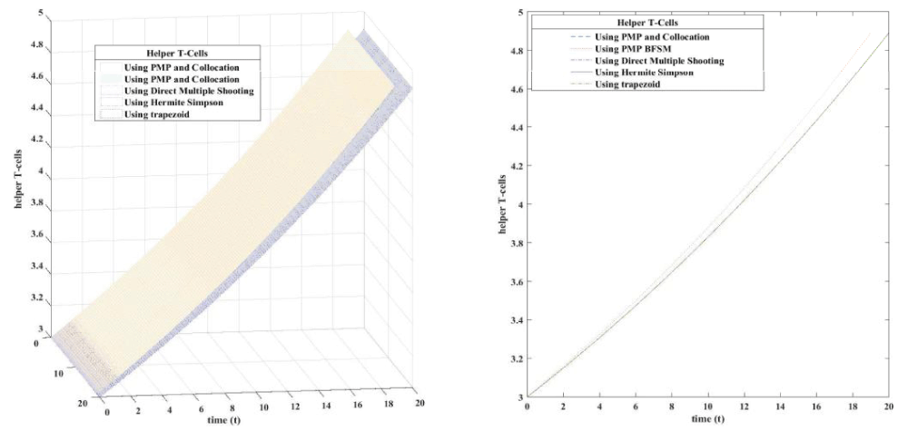
Figure 4.2: Helper T cells using 3D plot (left figure) and 2D plot (right figure).


Download Image

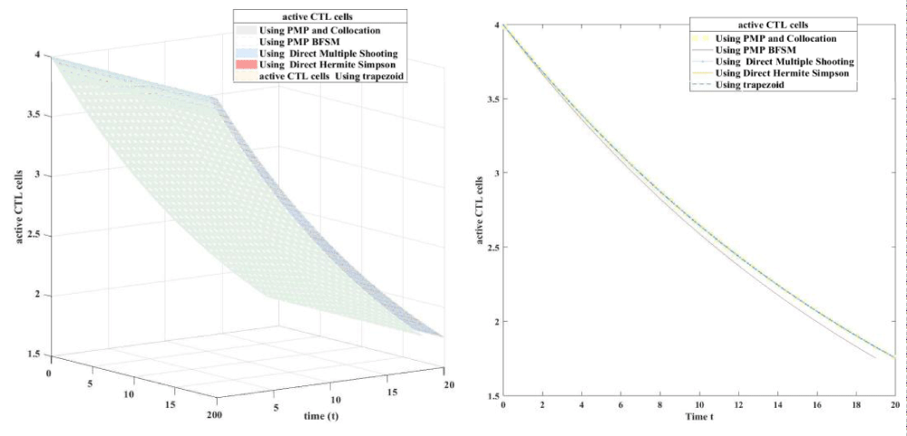
Figure 4.3: Active CTL using 3D plot (left figure) and 2D plot (right figure).


Download Image

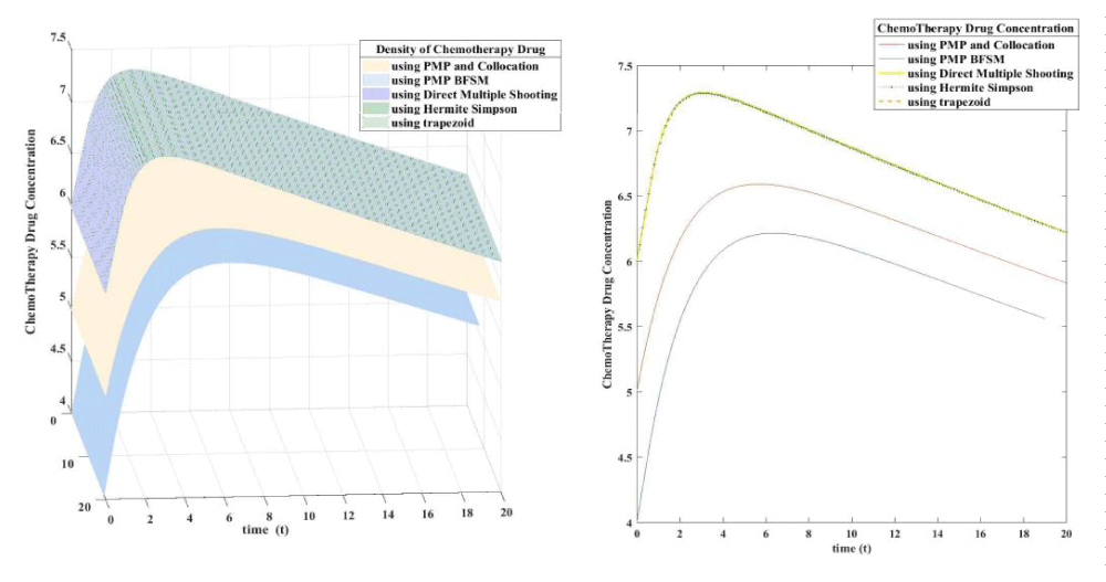
Figure 4.4:Density of Chemo Therapy Drug (3D plot) left side, (2D plot) right side.


Download Image

Figure 4.5: Control Plot using different methods.


Download Image

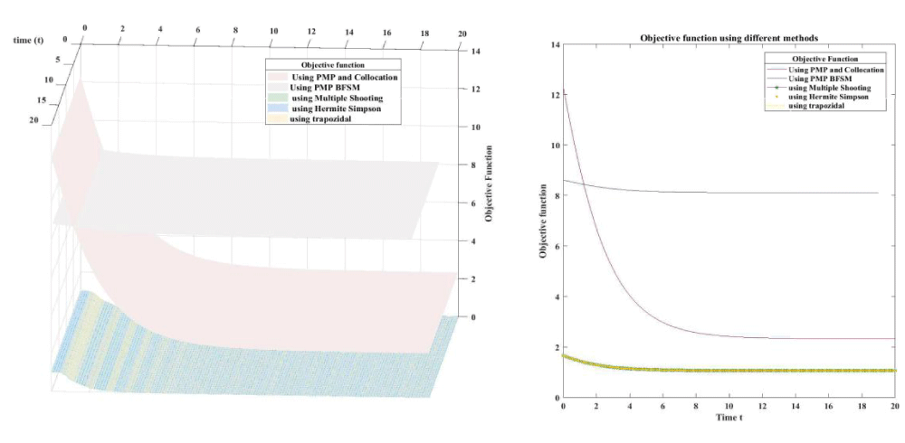
Figure 4.6: Objective Function Using different methods.


Download Image

Figure 4.7: State Error for Multiple Shooting Method.


Download Image

Figure 4.8: State Error for Hermite Simpson Method.


Download Image

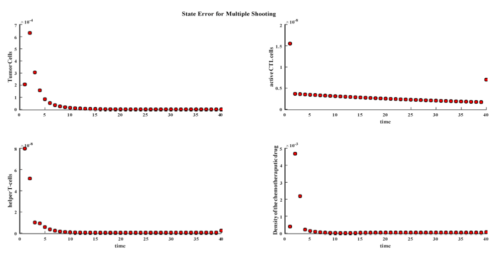
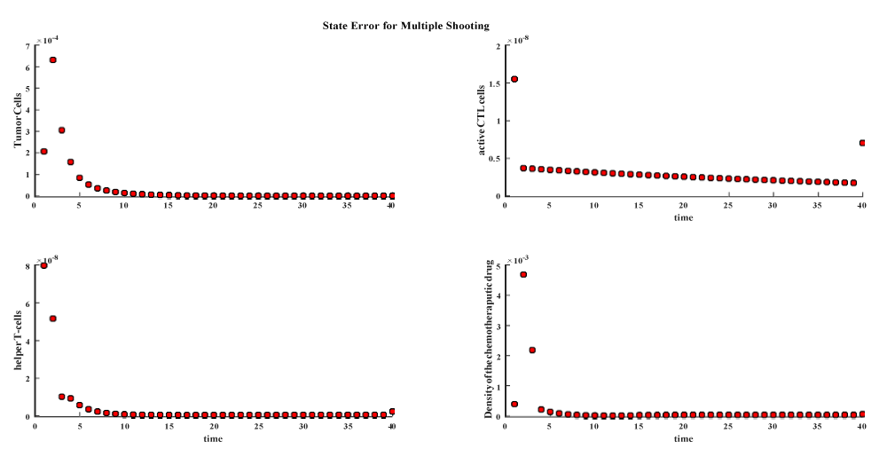
Figure 4.9: State Error for Direct Multiple Shooting Method.


Download Image

Figure 4.10: dx/dt - f(t,x,u) for Multiple Shooting.


Download Image

Figure 4.11: dx/dt - f(t,x,u) for Hermite Simpson.


Download Image

Figure 4.12: dx/dt - f(t,x,u) for trapezoid.

Table 2: Objective function values for different methods.
Method Objective Function J at tf value
Direct Multiple Shooting 1.067535615031329
Hermit Simpson DT 1.065628747428853
Trapezoidal DT 1.532368800622538
Pontryagin Maximum Principle and 3rd Lobotto collocation 2.324027433971033
Pontryagin Maximum principle and BFSM 8.118443453241154
Table 3: Different Comparsion merits for the direct method.
Method Name

Absolute local error

NLP iteration number

NLP time

Direct Multiple Shooting 0.004675646596448 60 9.305698207820010
Hermit Simpson
DT
7.125004407381137e-04 35 2.210647539360693
Trapezoidal DT 0.039534796829716 80 1.645410588354529

In all the previous figures the direct methods achieve better results than indirect methods. The values of controls and number of tumor cells made the big differences in the objective function of the theses methods. The number of tumor cells is lower in direct method than indirect methods also direct methods achieve better control than indirect method the following table shows the value of objective function for five different methods.

Since the direct methods achieve better results than indirect method this motivate us to give more insight into direct methods through new merits such as discretization error, absolute local error, number of NLP iterations, NLP time the following table gives the values of the previous merits for the methods of direct methods only.

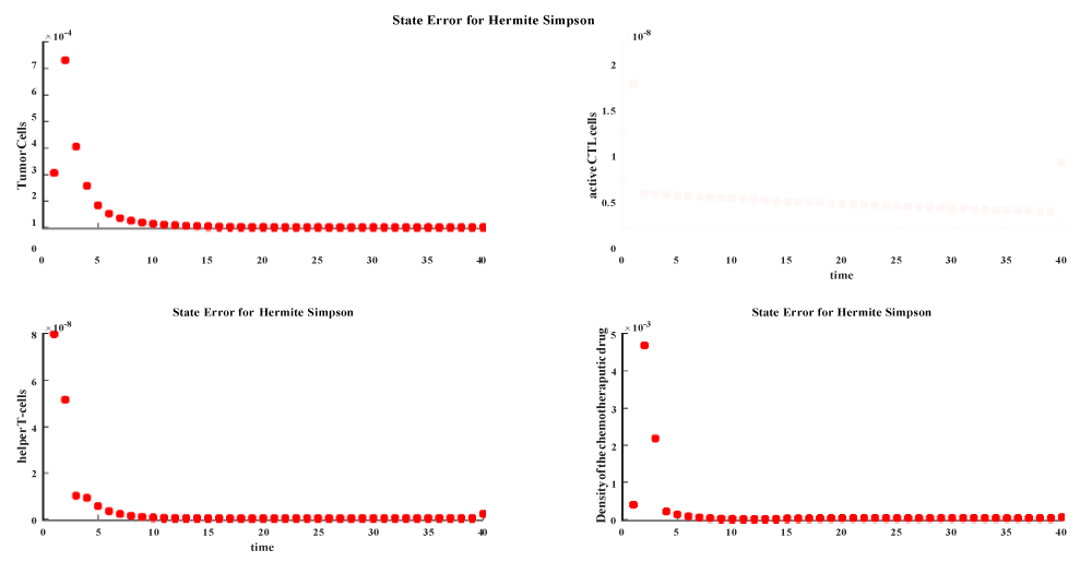
Within the direct method apart from indirect methods the results are butter in both Hermite Simpson DT and direct multiple shooting is butter than the trapozidal since both two methods represented by polynomials, the Hermite Simpson’s DT is better than the Trapezoidal DT since Hermite Simpson’s DT uses a higher order polynomial than trapezoidal DT which is an agreement with the concept of (p-method), for more details see [29], the hermite Simpson is the most accurate method on the price of time.

The following plots shows the different discretization errors and state errors for the three method.

In this article five numerical techniques to study the tumor immune dynamic optimization model are discussed, these methods are indirect method in which the resulting TPBVP is studied by collocation method, and by the backward forward sweep method and direct methods which are multiple shooting method, trapezoid direct collocation method, Hermite-Simpson’s direct collocation. Many studies claim that indirect methods have drawbacks. The two major drawbacks are that the differential equations obtained are often difficult to solve due to strong nonliterary and instability and also define a guess initial solution for the Lagrangian multiplier. As a matter of fact, these variables do not have a physical meaning, this leads to problems in the definition of an initial guess solution to start the algorithm. Another problem that it is necessary to take into account in the resolution of a BVP is that the existence and uniqueness of solution is not guaranteed as in an initial value problem. Each problem may have a unique solution, several solutions or no solution at all. By comparing different methods both in direct and indirect methods we can claim that direct method can be used to get better results than indirect method and it is easy to implement. A question that is needed to be answered is how to choose the discretization method among different methods related to direct method to get the best results this question can be a future work.

  1. Gibbs WW. Untangling the roots of cancer. Scientific America. 2003.
  2. Abbas AK, Lichtman AH, Pillai S. Cellular and molecular immunology. Saunders Elsevier. 2014.
  3. Curiel T. Tregs and rethinking cancer immunotherapy. Journal of Clinical Investigation. 2007; 117: 1167-1174. PubMed: https://www.ncbi.nlm.nih.gov/pubmed/17476346
  4. Kirschner D, P Panetta. Modeling immuno therapy of the tumor–immune interaction. Journal of Mathematical Biology. 1998; 37: 235-252. PubMed: https://www.ncbi.nlm.nih.gov/pubmed/9785481
  5. Kirschner DE, TL Jackson, JC Arciero. A mathematical model of tumorimmune evasion and siRNA treatment. Discrete and continous dynamical systems series- B. 2003; 37: 39-58.
  6. K Leon, K Garcia, J Carneiro. A Lage. How regulatory CD25(+)CD4(+) T cells impinge on tumor immunobiology? On the existence of two alternative dynamical classes of tumors. Journal of Theoretical Biology. 2007; 247: 122-137.
  7. De Pillis LG, Radunskaya AE. Mixed immunotherapy and chemotherapy of tumors: modeling, applications and biological interpretations. Journal of Theoretical Biology. 2006; 238.
  8. Schattlera H, Urszula L. Optimal Control for Mathematical Models of Cancer Therapies. Springer Publishing Co., USA. 2015.
  9. Sharma S, Samanta GP. Dynamical Behaviour of a Tumor-Immune System with Chemotherapy and Optimal Control. Journal of Nonlinear Dynamics. 2013: 1-13, 2013.
  10. Sweilam NH, Al-Ajami TM. Legendre spectral-collocation method for solving some types of fractional optimal control problems. Journal of Advanced Research, 2015; 393-403. PubMed: https://www.ncbi.nlm.nih.gov/pubmed/26257937
  11. García-Heras J, Soler M, Sáez FJ. A Comparison of Optimal Control Methods for Minimum Fuel Cruise at Constant Altitude and Course with Fixed Arrival Time. Procedia Engineering. 2014; 80:231-244.
  12. Rao AV, Benson DA, Darby C, Patterson MA, Francolin C, et al. Algorithm 902: GPOPS, A MATLAB software for solving multiple-phase optimal control problems using the gauss pseudospectral method. ACM Transactions on Mathematical Software (TOMS), 2010; 37: 1-39.
  13. Biral F, Bertolazzi E, Bosetti P. Notes on Numerical Methods for Solving Optimal Control Problems. IEEJ Journal of Industry Applications. 2015; 5:154-166
  14. Betts JT. A Survey of Numerical Methods for Trajectory Optimization. Control and Dynamics. 1998; 21:193-207.
  15. Rao AV. A survey of numerical methods for optimal control. Advances in the Astronautical Sciences. 2009; 135: 497-528.
  16. Joshi HR. Optimal control of an HIV immunology model. Optimal Control Applications and Methods. 2002; 23: 199-213.
  17. Zaman G, Han Kang Y, Jung IH. Stability analysis and optimal vaccination of an SIR epidemic model. BioSystems. 93: 240-249. 2008. PubMed: https://www.ncbi.nlm.nih.gov/pubmed/18584947
  18. Pillis LG, Radunskaya AE. A mathematical model of immune response to tumor invasion. MIT. 2003; 1661-16668.
  19. De Pillis LG, W Gu, Fister KR, Head T, Maples K, et al. Chemotherapy for tumors: An analysis of the dynamics and a study of quadratic and linear optimal controls. Mathematical Biosciences. 2007; 209: 292-315.
  20. Bellman RE. Dynamic Programming. Courier Corporation. 2003.
  21. Pontryagin LS. Mathematical Theory of Optimal Processes. CRC Press. March 1987.
  22. Anita S, Arnautu V, Capasso V. An introduction to optimal control problems in life sciences and economics: from mathematical models to numerical simulation with MATLAB®. Modeling and simulation in science, engineering and technology. Birkhäuser. New York. 2011.
  23. Sweilam NH, AL-Mekhla M. On the Optimal Control for Fractional Multi-Strain TB Model. Optimal Control, Applications and Methods. 2016.
  24. Karush W. Minima of Functions of Several Variables with Inequalities as Side Constraints. Ph.D. Department of Mathematics. University of Chicago. Chicago. 1939
  25. H Kuhn, A Tucker. Nonlinear Programming. 1951; 481-492, California. University of California Press. Berkeley.
  26. Bryson AE, Ho YC. Applied optimal control. Hemisphere Publication Corporation. 1975.
  27. Aktas Z, Stetter HJ. A classification and survey of numerical methods for boundary value problems in ordinary differential equations. International journal for numerical methods in engineering. 1977; 11: 771-796.
  28. Shampine LF, Gladwell I, Thompson S. Solving ODEs with MATLAB. Cambridge University Press. 2003.20.
  29. Lenhart S and Workman JT. Optimal Control Applied to Biological Models. Chapman & Hall/CRC Mathematical and Computational Biology. CRC Press. Taylor & Francis Group. 2007.
  30. Mitter SK. The successive approximation method for the solution of optimal control problems. Automotica. 1996; 3:135-149.
  31. Hackbusch W. A numerical method for solving parabolic equations with opposite orientations. Computing. 1978; 20: 229-240.
  32. Victor VM. Practical Direct Collocation Methods for Computational Optimal Control. In Modeling and Optimization in Space Engineering. Volume 73 of Springer Optimization and Its Applications. Springer New York. 2013; 33-60.
  33. Chachuat B. Nonlinear and Dynamic Optimization: From Theory to Practice - IC-32: Spring Term. EPFL. 2009.
  34. Binder T, Blank L, Bock HG, Bulirsch R, Dahmen W, et al. Introduction to Model Based Optimization of Chemical Processes on Moving Horizons. In Introduction to Model Based Optimization of Chemical Processes on Moving Horizons. Springer Berlin Heidelberg. 2001; 295-339.
  35. Bock H, Plitt K. A multiple shooting algorithm for direct solution of optimal control problems. In 9th IFAC. Pergamon Press. 1984; 242-247.
  36. Diehl M, Findeisen R, Schwarzkopf S, Uslu I, Allgöwer F, et al. An Efficient Algorithm for Nonlinear Model Predictive Control of Large-Scale Systems Part I: Description of the Method. At-Automatisierungstechnik Methoden und Anwendungen der Steuerungs-, Regelungs-und Informationstechnik, 2002; 50: 557.
  37. Dickmanns ED, Well KH. Approximate solution of optimal control problems using third order hermite polynomial functions. In Marchuk GI, editor. Optimization Techniques IFIP Technical Conference Novosibirsk, number 27 in Lecture Notes in Computer Science, pages. Springer Berlin Heidelberg. 1974; 158-166.
  38. Törn A, Žilinskas A, Goos G, Hartmanis J, Barstow D, et al. Global Optimization, volume 350 of Lecture Notes in Computer Science. Springer Berlin Heidelberg. Berlin. Heidelberg. 1989.
  39. Biegler LT. Nonlinear programming: concepts, algorithms, and applications to chemical processes. Number 10 in MOS-SIAM series on optimization. SIAM. Philadelphia. 2010.
  40. Betts JT. Practical methods for optimal control and estimation using nonlinear programming. Advances in design and control. Society for Industrial and Applied Mathematics. Philadelphia. 2nd edition. 2010.
  41. Matthew PK. Transcription Methods for Trajectory Optimization A beginners tutorial. Technical report. Cornell University. 2015.
  42. E Hairer, Norsett SP, Wanner G. Solving Ordinary Differential Equations I Nonstiff Problems. Springer-Verlag Berlin Heidelberg, 2008.